## Warning in .GitClone(pID, scriptID): Cloning into '/home/runner/work/_temp/Library/revbayes-repos/104_by_n_ki'...
##   fatal: could not read Username for 'https://github.com': terminal prompts disabled
## Warning in ConnectSSH(): sshLogin environment variable not set in ConnectSSH()
.cache <- system.file("extdata/stationarity_data.RData", package = "neotrans")

if (.sim_available) {
  p1 <- vapply(KiProjects(), function(pID) {
    neo <- InfNeo(pID)
    p1Taxa <- neo[["1"]] / (neo[["0"]] + neo[["1"]])
    p1Obs <- sum(neo[["1"]]) / sum(neo[["0"]], neo[["1"]])

    p1Sim <- Simulated01s(pID, "by_n_ki")
    if (length(p1Sim) < 2) {
      return(rep(NA_real_, 1 + 6 + 6))
    }
    cli::cli_progress_message("{pID}: Compute Sim stats")
    p1Sim <- p1Sim["1", ] / colSums(p1Sim)
    c(obs = p1Obs,
      obs = quantile(p1Taxa, c(0.025, 0.25, 0.5, 0.75, 0.975), na.rm = TRUE),
      obs.mad = mad(p1Taxa),
      sim = quantile(p1Sim, c(0.025, 0.25, 0.5, 0.75, 0.975), na.rm = TRUE),
      sim.mad = mad(p1Sim))
  }, double(1 + 6 + 6)); cli::cli_progress_done()

  ns1 <- vapply(KiProjects(), function(pID) {
    c(obs1 = InfNeo(pID)[[c("p", "1")]],
      obs1 = quantile(InfNeo(pID)[["p1"]], c(0.25, 0.75), na.rm = TRUE),
      root1 = ExistingResults(pID, "ns_n_ki")[["parameters"]][
        , "root_freqs.2."] %||% rep(NA_real_, 6))
  }, double(1 + 2 + 6))

  nsP1AtStat <- vapply(KiProjects(), function(pID) {
    p1Sim <- Simulated01s(pID, "ns_n_ki", "stat")
    if (length(p1Sim) < 2) {
      return(rep(NA_real_, 6))
    }
    p1Sim <- p1Sim["1", ] / colSums(p1Sim)
    c(sim = quantile(p1Sim, c(0.025, 0.25, 0.5, 0.75, 0.975), na.rm = TRUE),
      sim.mad = mad(p1Sim))
  }, double(6)); cli::cli_progress_done()

  nsP1AtObs <- vapply(KiProjects(), function(pID) {
    p1Sim <- Simulated01s(pID, "ns_n_ki", "obs")
    if (length(p1Sim) < 2) {
      return(rep(NA_real_, 6))
    }
    p1Sim <- p1Sim["1", ] / colSums(p1Sim)
    c(sim = quantile(p1Sim, c(0.025, 0.25, 0.5, 0.75, 0.975), na.rm = TRUE),
      sim.mad = mad(p1Sim))
  }, double(6)); cli::cli_progress_done()

  rootFreqCf <- vapply(KiProjects(), function(pID) {
    par <- ExistingResults(pID, "ns_n_ki")[["parameters"]]
    if (is.null(par)) {
      MakeSlurm(pID, "ns_n_ki", ml = FALSE)
      return(rep(NA_real_, 2))
    }
    n <- 1 / par["50%", "rate_loss"] # confusingly named?
    c(pi0 = 1 / (1 + n), # Probability of absence at stationary distribution
      a0 = par["50%", "root_freqs.1."])
  }, double(2))

  delta <- rootFreqCf["a0", ] - rootFreqCf["pi0", ]
} else {
  load(.cache) # loads p1, ns1, nsP1AtStat, nsP1AtObs, rootFreqCf, delta, kiNeoChar
}

.meta <- Metadata()
kiNeoChar <- .meta$nChar["neo", KiProjects()]
OutputPlot("stationarity", 7.2, 7, function() {
  layout(rbind(1:2, 3:4, c(5, 5)), heights = c(1, 1, 1/4))
  par(mar = c(4.2, 4.2, 0.4, 0.4))

  # Results of posterior predictive samples.
  # These are not particularly illuminating.
  ColErrPlot(
    "Observed Pr(present)", p1["obs", ], p1["obs.25%", ], p1["obs.75%", ],
    "Pr(present), NstN, stationary root",
    nsP1AtStat["sim.50%", ], nsP1AtStat["sim.2.5%", ], nsP1AtStat["sim.97.5%", ],
    lgdTitle = "Characters", colBy = kiNeoChar,
    text = TRUE)

  ColErrPlot(
    "Observed Pr(present)", p1["obs", ], p1["obs.25%", ], p1["obs.75%", ],
    "Pr(present), NstN, inferred root frequencies",
    nsP1AtObs["sim.50%", ], nsP1AtObs["sim.2.5%", ], nsP1AtObs["sim.97.5%", ],
    lgdTitle = "Characters", colBy = kiNeoChar,
    text = TRUE)

  postPred <- data.frame(
    stat_root_fqs = nsP1AtStat["sim.50%", ],
    obs_root_fqs = nsP1AtObs["sim.50%", ],
    stat_obs = nsP1AtObs["sim.50%", ] - nsP1AtStat["sim.50%", ])

  SpindlePlot(postPred)


  ColErrPlot(
    "Observed Pr(present)", p1["obs", ], p1["obs.25%", ], p1["obs.75%", ],
    "Pr(present), NstN, inferred root frequencies - stationary root",
    nsP1AtObs["sim.50%", ] - nsP1AtStat["sim.50%", ],
    nsP1AtObs["sim.50%", ] - nsP1AtStat["sim.50%", ],
    nsP1AtObs["sim.50%", ] - nsP1AtStat["sim.50%", ],
    asp = NULL, ylim = 0.5 * c(-1, 1), line = "h",
    lgdTitle = "Characters", colBy = kiNeoChar,
    text = TRUE)

  ColErrPlot(
    "Root Pr(present)",
    ns1["root1.50%", ], ns1["root1.2.5%", ], ns1["root1.97.5%", ],
    "Leaf Pr(present)",
    ns1["obs1", ], ns1["obs1.25%", ],  ns1["obs1.75%", ],
    lgdTitle = "Characters", colBy = kiNeoChar, text = TRUE)

  ColErrPlot("Stationary Pr(present)",
             1 - rootFreqCf["pi0", ],
             1 - rootFreqCf["pi0", ],
             1 - rootFreqCf["pi0", ],
             "Excess Pr(present) at root relative to stationary distribution",
             delta, delta, delta,
             line = "h", ylim = c(-0.5, 0.5),
             col = kiNeoChar)

})
dStat <- p1["obs", ] - nsP1AtStat["sim.50%", ]
dObs <- p1["obs", ] - nsP1AtObs["sim.50%", ]

ColErrPlot("Difference in Pr(present), observed vs sim from stationary root",
           dStat, dStat, dStat,
           "Difference in Pr(present), observed vs sim from observed root",
           dObs, dObs, dObs,
           line = c("h", "v"), xlim = range(c(dStat, dObs), na.rm = TRUE),
           lgdTitle = "Characters", col = kiNeoChar, text= TRUE)
ColErrPlot(
  "Pr(present), NstN, inferred root frequencies",
  nsP1AtObs["sim.50%", ], nsP1AtObs["sim.2.5%", ], nsP1AtObs["sim.97.5%", ],
  "Pr(present), NstN, stationary root",
  nsP1AtStat["sim.50%", ], nsP1AtStat["sim.2.5%", ], nsP1AtStat["sim.97.5%", ],
  lgdTitle = "Characters", colBy = kiNeoChar,
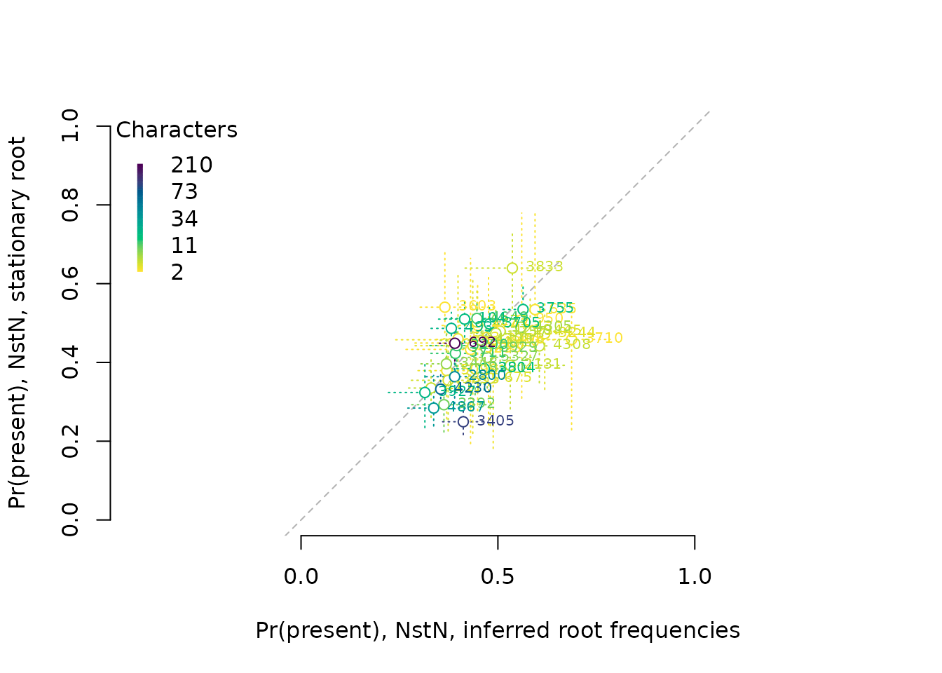
  text = TRUE)
ColErrPlot(
  "Leaf Pr(present)",
  ns1["obs1", ], ns1["obs1.25%", ],  ns1["obs1.75%", ],
  "Root Pr(present)",
  ns1["root1.50%", ], ns1["root1.2.5%", ], ns1["root1.97.5%", ],
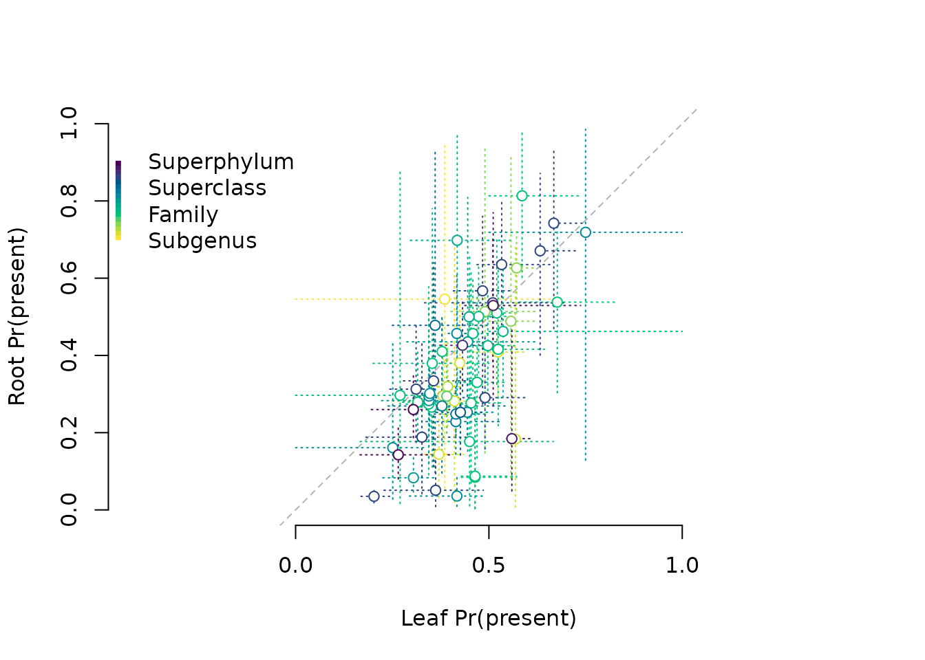
  colBy = droplevels(.meta$rank[KiProjects()]))
ColErrPlot(
  "Leaf Pr(present)",
  ns1["obs1", ], ns1["obs1.25%", ],  ns1["obs1.75%", ],
  "Root Pr(present)",
  ns1["root1.50%", ], ns1["root1.2.5%", ], ns1["root1.97.5%", ],
  lgdTitle = "Taxon",
  colBy = .meta$taxon[KiProjects()], pal = palette.colors(5)[-1])
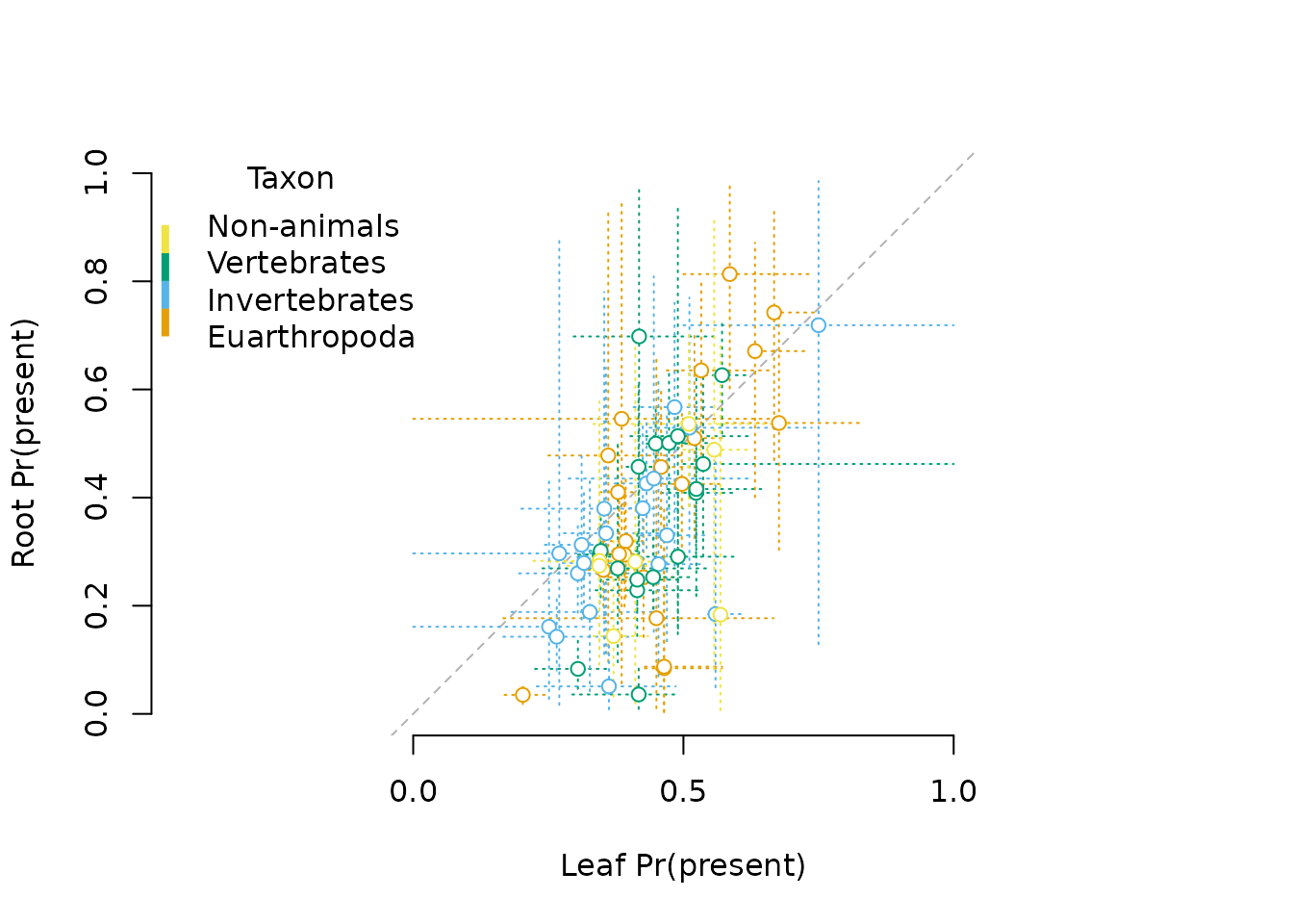
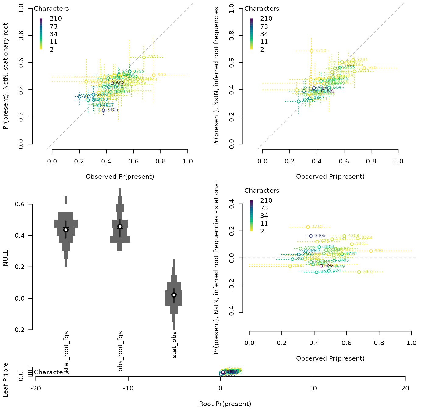
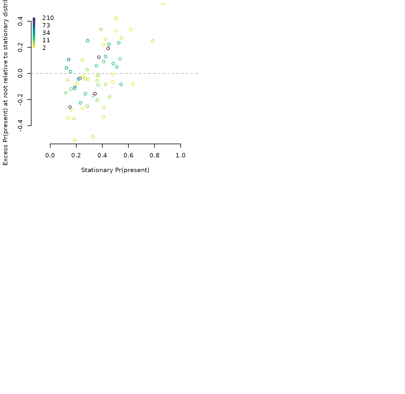
# The proportion of present states at the root deviates from the stationary distribution by > 0.1 in 20 of 64 datasets, and is 0.1 less than the stationary distribution in 20 datasets.
sum(delta > 0.1, na.rm = TRUE)
## [1] 20
sum(delta < -0.1, na.rm = TRUE)
## [1] 20
## [1] 64
OutputPlot("rootVsLeaf", 5, 5, function() {
  par(mar = c(4, 4.2, 0.4, 0.2), cex = 0.8)
  ColErrPlot(
    expression("Pr(" * italic("present") * ") at root"),
    ns1["root1.50%", ], ns1["root1.2.5%", ], ns1["root1.97.5%", ],
    expression("Excess Pr(" * italic("present") * ") at leaves"),
    ns1["obs1", ] - ns1["root1.50%", ],
    ns1["obs1", ] - ns1["root1.97.5%", ],
    ns1["obs1", ] - ns1["root1.2.5%", ],
    ylim = c(-0.5, 0.5), lgdPos = "bottomleft",
    line = "h",
    lgdTitle = "Neomorphic codings\n per taxon",
    colBy = .meta$nNeoCoded[KiProjects()] / .meta$nTaxa[KiProjects()],
    text = FALSE)
  abline(v = 0.5, lty = "dashed", col = "grey70")

  text(1.0, 0.35, "More presences at leaves than root \U2191", pos = 2)
  text(1.0, 0, "Stationary distribution", pos = 2)
  text(1.0, -0.35, "More absences at leaves than root \U2193", pos = 2)
})
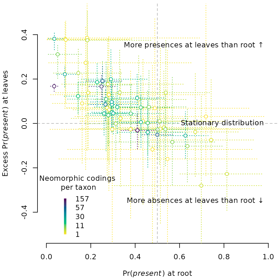
moreAtLeaves <- ns1["obs1", ] - ns1["root1.97.5%", ] > 0
moreAtRoot <- ns1["obs1", ] - ns1["root1.2.5%", ] < 0
sum(moreAtLeaves, na.rm = TRUE)
## [1] 15
sum(moreAtRoot, na.rm = TRUE)
## [1] 1
## [1] 64
signif(median(ns1["root1.50%", moreAtLeaves], na.rm = TRUE), 2)
## [1] 0.14
signif(max(ns1["root1.97.5%", moreAtLeaves], na.rm = TRUE), 2)
## [1] 0.48
leafExcess <- ns1["obs1", !is.na(moreAtLeaves)] -
  ns1["root1.50%", !is.na(moreAtLeaves)]
leafProj <- names(leafExcess)
meta <- data.frame(
  leafExcess,
  nChar = colSums(.meta$nChar[, leafProj]),
  obsP1 = ns1["obs1", leafProj],
  nTrans = .meta$nChar["trans", leafProj],
  nNeo = .meta$nChar["neo", leafProj],
  logNTRatio = log(.meta$nChar["neo", leafProj] / .meta$nChar["trans", leafProj]),
  neoPerTax = .meta$nChar["neo", leafProj] / .meta$nTaxa[leafProj],
  taxon = .meta$taxon[leafProj],
  rank = .meta$rank[leafProj],
  nTaxa = .meta$nTaxa[leafProj]
)

leafPredictors <- c("nNeo", "obsP1", "logNTRatio", "neoPerTax", "taxon", "rank",
                    "nTaxa")
vsurfBF <- VSURF::VSURF(meta[, leafPredictors], leafExcess, verbose = FALSE)
predBF <- leafPredictors[vsurfBF[["varselect.pred"]]]
if (!length(predBF)) {
  predBF <- leafPredictors[vsurfBF[["varselect.interp"]]]
}
message(paste0(predBF, collapse = ", "))
## neoPerTax, logNTRatio
## randomForest 4.7-1.2
## Type rfNews() to see new features/changes/bug fixes.
rfBF <- randomForest(meta[, predBF, drop = FALSE], leafExcess,
                     ntree = 10000, importance = TRUE)
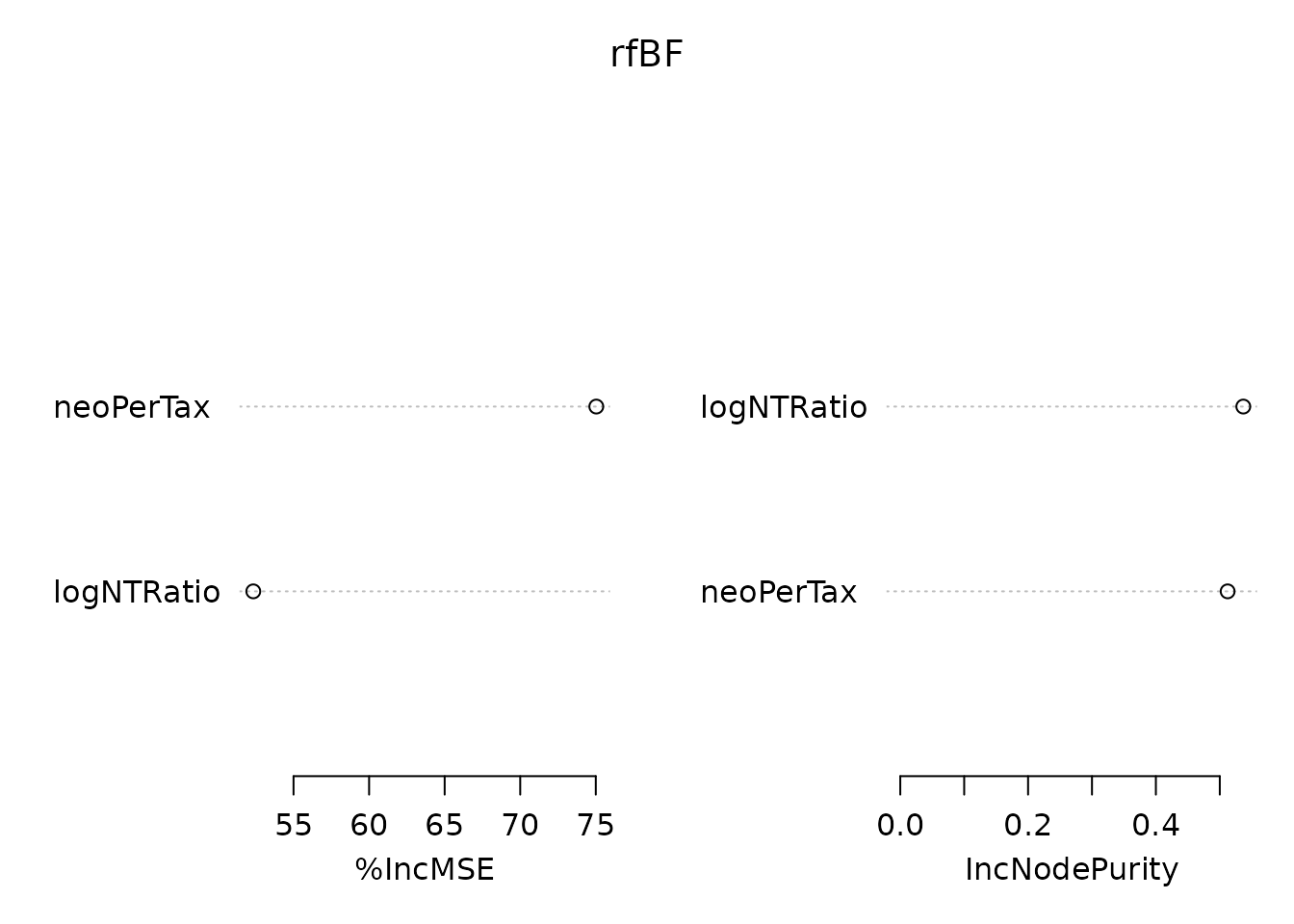
importance(rfBF)
##             %IncMSE IncNodePurity
## neoPerTax  75.03455     0.5122981
## logNTRatio 52.33681     0.5368185