Parameter analysis
Martin R. Smith martin.smith@durham.ac.uk
2026-03-06
Source:vignettes/parameter-analysis.Rmd
parameter-analysis.RmdAnalysis of parameter values and properties.
Prepare analysis environment
library("randomForest")
library("neotrans")

.meta <- Metadata()
.config <- Config()
epsBF <- log(10) # "Strong" support, per Jeffries 1939
Models with a free t parameter
The parameter t is the ratio of the evolution rate of transformational characters to that of neomorphic characters; fixing t = 1 assumes both partitions evolve at the same rate.
Review accuracy of marginal likelihood estimates
Before interpreting Bayes factors we verify that stepping-stone and path-sampling marginal likelihood estimates agree, as large discrepancies would undermine model comparisons.
modelsT <- c("by_ki", "by_n_ki", "by_t_ki", "by_nt_ki", "rm_by_t_ki")
marginals <- GetMarginals(KiProjects(), modelsT)
stdErr <- attr(marginals, "stdErr")
mds <- MarginalDiffs(KiProjects(), modelsT)
hist(abs(mds), breaks = ceiling(max(abs(mds), na.rm = TRUE) * 2), xpd = NA)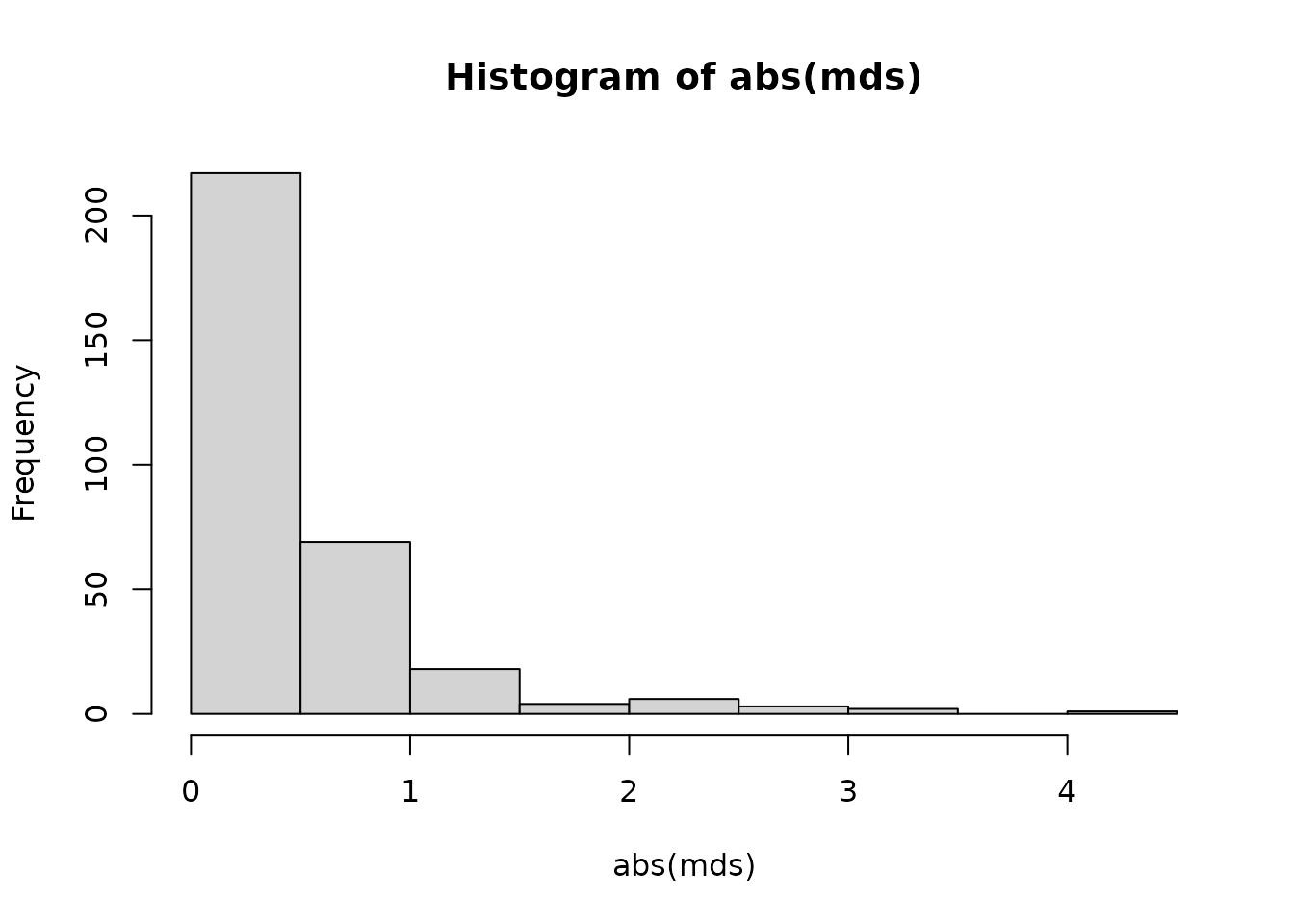
plot(stdErr, mds, frame.plot = FALSE, xlab = "Standard error of estimate",
     ylab = "Difference, stepping stone vs path sampling estimates",
     col = ModelCol(modelsT), pch = 16)
abline(h = 0, lty = "dashed", col = "grey70")
abline(0, 1, lty = "dashed", col = "grey70")
legend("topleft", ModelLabel(modelsT), pch = 16, col = ModelCol(modelsT),
       bty = "N")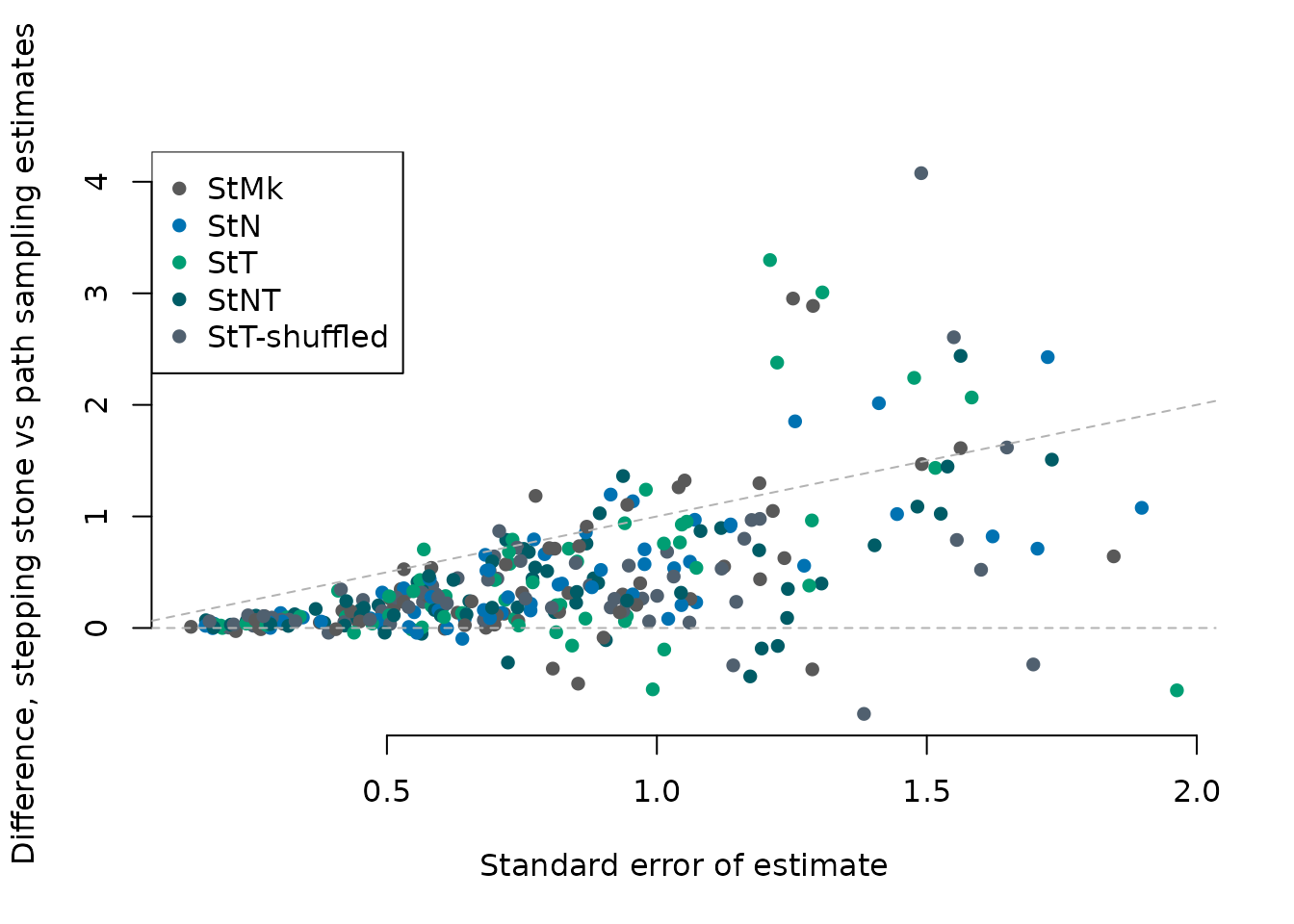
When is a partitioned model preferred?
Using a threshold of log(BF) > log(10) (Jeffreys’ ‘strong’ evidence), we identify datasets where a free t is decisively favoured or disfavoured, and plot these against the character composition of each dataset.
part <- EvaluatePartitioning(marginals)## by_t is >eps better than unpartitioned in 15 / 64 projects.## by_t is >eps better than rm_by_t in 13 / 15 of these.## rm_by_t is best model by >eps in 3 / 64
tSupport <- part["by_t_ki", ] - part["by_ki", ]
tErr <- .DiffErr(stdErr["by_t_ki", ], stdErr["by_ki", ])
tFitsBest <- .OutwithError(tSupport, tErr)
sum(tFitsBest)
## [1] 15
tCol <- hcl.colors(6, "Red-Green")[c(2, 2, 5, 5)][
  cut(tSupport, breaks = c(-Inf, -epsBF, 0, epsBF, Inf))]

par(mar = c(4, 4, 0.4, 0.4))
plot(.meta$nChar["trans", ], .meta$nChar["neo", ],
     pch = ifelse(tFitsBest | .OutwithError(-tSupport, tErr), 16, 1),
     col = tCol,
     xlab = "Transformational characters", ylab = "Neomorphic characters",
     log = "xy",
     asp = 1, frame.plot = FALSE)
abline(0, 1, lty = "dashed")
legend("topleft", bty = "n", title = expression(italic(t) ~ "parameter:"),
       legend = c("Free preferred",
                  "Fixed preferred",
                  paste0("BF > ", signif(epsBF, 3)),
                  paste0("BF < ", signif(epsBF, 3))),
       pch = c(15, 15, 16, 1),
       pt.cex = 1.2,
       col = c(hcl.colors(6, "Red-Green")[5],
               hcl.colors(6, "Red-Green")[2],
               "grey10", "grey10"))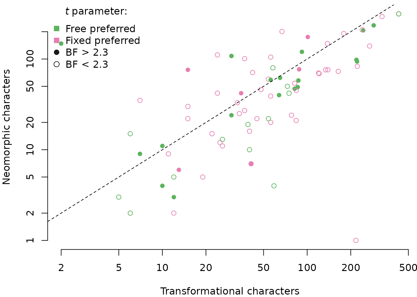
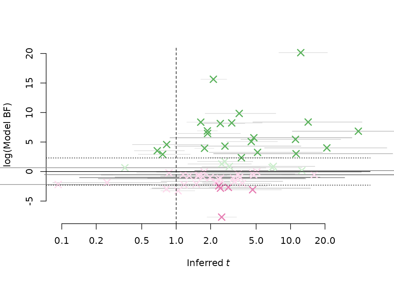
We next examine the posterior distribution of t under the best-fitting stationary model for each dataset, and test whether inferred values differ significantly from one.
# Compare estimated values of t
bestTModel <- ifelse(marginals["by_t_ki", ] > marginals["by_nt_ki", ],
                     "by_t_ki", "by_nt_ki")
tProjects <- names(bestTModel)[!is.na(bestTModel)]

# Estimated value of t using the best available stationary model
stationaryT <- sapply(tProjects, function(pID) {
  exRes <- ExistingResults(pID, bestTModel[[pID]], checkRemote = FALSE)
  if (exRes[["convergence"]][["ess"]] < .config$essThreshold) {
    message("Extending run for ", pID, "_", bestTModel[pID])
    MakeSlurm(pID, bestTModel[pID], ml = FALSE)
  }
  res <- exRes[["parameters"]][, "rate_neo"]
  # partition_rate := [ rate_neo / (1 + rate_neo), (1 / (1 + rate_neo)) ]
  # MS defines t = rate_t / rate_n

  if (is.null(res)) {
    message("Need results for ", pID, "_", bestTModel[pID])
    RevBayes(pID, bestTModel[pID])
    MakeSlurm(pID, bestTModel[pID], ml = FALSE)
    setNames(rep(NA, 6), c("2.5%", "25%", "50%", "75%", "97.5%", "mad"))
  } else {
    # Convert from rate_neo to rate_trans
    1 / res
  }
})
shapiro.test(log(stationaryT["50%", ]))
##
## Shapiro-Wilk normality test
##
## data: log(stationaryT["50%", ])
## W = 0.96209, p-value = 0.04682##
## One Sample t-test
##
## data: log(stationaryT["50%", ])
## t = 7.6759, df = 63, p-value = 1.317e-10
## alternative hypothesis: true mean is not equal to 0
## 95 percent confidence interval:
## 0.7189701 1.2250885
## sample estimates:
## mean of x
## 0.9720293## [1] 2.47## [1] 2.28## [1] 7.58## [1] 2.64## [1] 1.013
# Because of the conversion, the 2.5%ile is "high" and the 97.5%ile is "low"
message(
  "Median: ", signif(median(stationaryT["50%", ], na.rm = TRUE), 3),
  " (= 1/", signif(1 / median(stationaryT["50%", ], na.rm = TRUE), 3),
  "), mad ", signif(mad(stationaryT["50%", ], na.rm = TRUE), 3),
  "; LogMean: ", signif(exp(mean(log(stationaryT["50%", ]), na.rm = TRUE)), 3),
  ", sd ", signif(exp(sd(log(stationaryT["50%", ]), na.rm = TRUE)), 3)
)
## Median: 2.47 (= 1/0.405), mad 1.64; LogMean: 2.64, sd 2.75
tNotOne <- stationaryT["97.5%", ] > 1 | stationaryT["2.5%", ] < 1
message("Different from 1: ", sum(tNotOne, na.rm = TRUE),
        " / ", sum(!is.na(tNotOne)), ": ",
        sum(stationaryT["97.5%", ] > 1, na.rm = TRUE), " > 1; ",
        sum(stationaryT["2.5%", ] < 1, na.rm = TRUE), " < 1")
## Different from 1: 36 / 64: 35 > 1; 1 < 1
ntBest <- (bestTModel == "by_nt_ki")[!is.na(bestTModel)]
tModelBF <- setNames(numeric(length(tProjects)), tProjects)
tModelBF[ntBest] <- marginals["by_nt_ki", tProjects[ntBest]] -
  marginals["by_n_ki", tProjects[ntBest]]
tModelBF[!ntBest] <- marginals["by_t_ki", tProjects[!ntBest]] -
  marginals["by_ki", tProjects[!ntBest]]
tColBin <- ifelse(tModelBF < 0,
                  ifelse(tModelBF < pmin(-epsBF, -tErr), 1, 2),
                  ifelse(tModelBF > pmax(epsBF, tErr), 4, 3))
tCol <- hcl.colors(6, "Red-Green")[2:5][tColBin]

{
  par(mfrow = c(1, 1))
  plot(stationaryT["50%", ], tModelBF,
       xlab = expression("Inferred" ~ italic("t")), # under best stationary model
       ylab = "log(Model BF)", xpd = NA,
       frame.plot = FALSE, pch = 4, log = "x")
  confidenceCol <- gray.colors(256)
  iqr <- log(stationaryT["75%", ]) - log(stationaryT["25%", ])
  segments(stationaryT["2.5%", ], tModelBF, stationaryT["97.5%", ], xpd = NA,
           col = confidenceCol[cut(iqr, breaks = 256)])
  points(stationaryT["50%", ], tModelBF, col = tCol,
         pch = 4, cex = 1.5, lwd = 2)
  abline(v = 1, lty = 2)
  EpsLine()
}
Predict which projects will favour a free t
Variable selection via VSURF, followed by a random forest, identifies which dataset-level properties predict whether a free t is supported.
# Can we predict which projects will benefit from a free t parameter?
tProj <- names(tSupport)
tMeta <- data.frame(
  tSupport,
  nChar = colSums(.meta$nChar[, tProj]),
  nTrans = .meta$nChar["trans", tProj],
  nNeo = .meta$nChar["neo", tProj],
  logNTRatio = log(.meta$nChar["neo", tProj] / .meta$nChar["trans", tProj]),
  charPerTax = colSums(.meta$nChar[, tProj]) / .meta$nTaxa[tProj],
  taxon = .meta$taxon[tProj],
  rank = .meta$rank[tProj],
  nTaxa = .meta$nTaxa[tProj],
  tValue = log(t(stationaryT[, tProj]))
)

tPredictors <- c("nChar", "logNTRatio", "charPerTax", "taxon", "rank", "nTaxa",
                 "tValue.50.")
vsurfBF <- VSURF::VSURF(tMeta[, tPredictors], tSupport, verbose = FALSE)
predBF <- tPredictors[vsurfBF[["varselect.pred"]]]
if (!length(predBF)) {
  predBF <- tPredictors[vsurfBF[["varselect.interp"]]]
}
cat(paste0(predBF, collapse = ", "))
## tValue.50., charPerTax, nChar, logNTRatio
rfBF <- randomForest(tMeta[, predBF, drop = FALSE], tSupport,
                     ntree = 10000, importance = TRUE)
importance(rfBF)
## %IncMSE IncNodePurity
## tValue.50. 64.27070 337.7876
## charPerTax 39.75346 264.0440
## nChar 36.89633 313.9492
## logNTRatio 44.69695 257.2419
varImpPlot(rfBF, frame.plot = FALSE)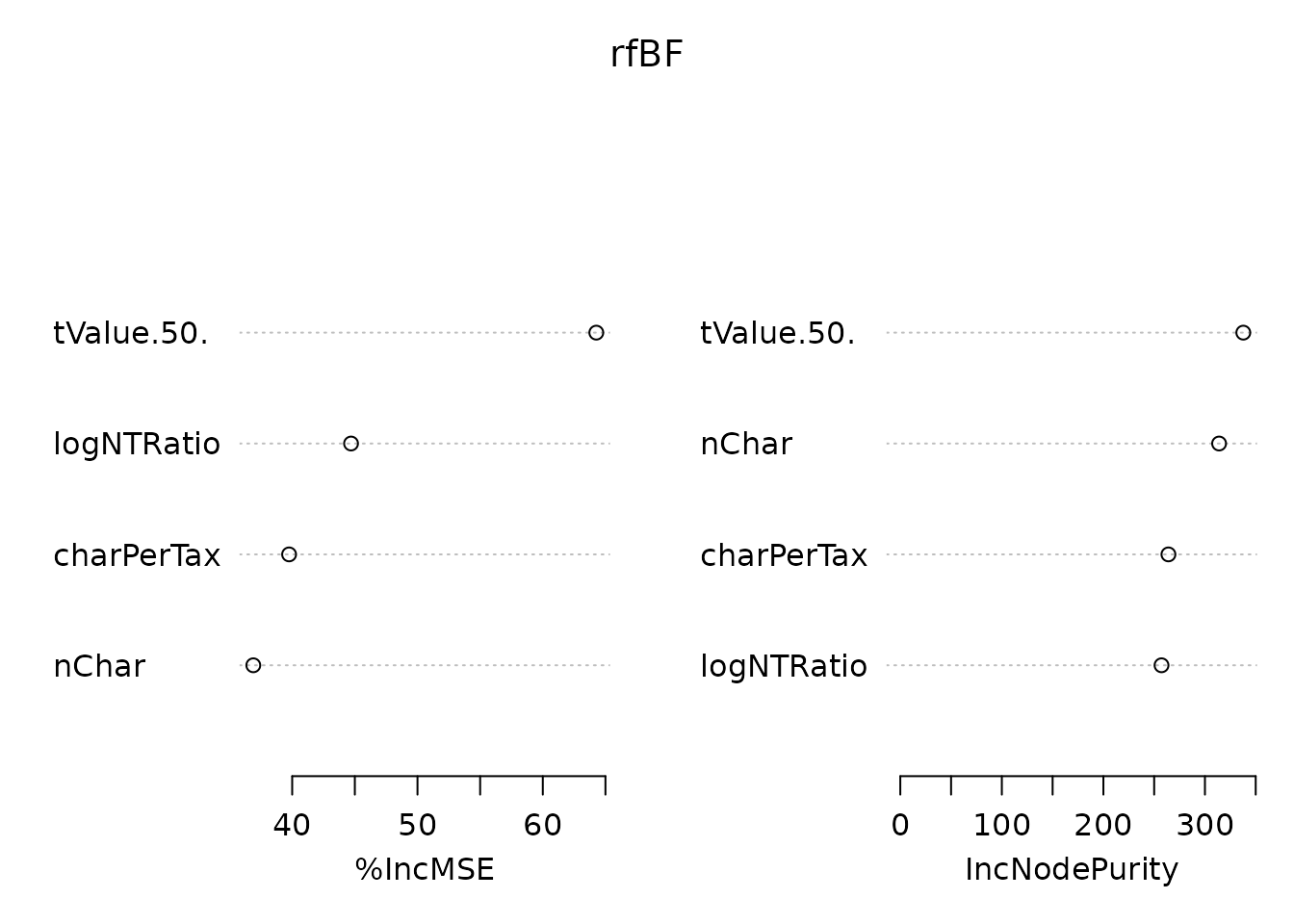
nPred <- length(predBF)

par(mfrow = c(nPred, 2))
for (predictor in predBF) {
  partialPlot(rfBF, tMeta[, tPredictors], as.character(predictor),
              rug = TRUE, frame.plot = FALSE, main = "",
              xlab = Decrypt(predictor),
              ylab = "Impact on predicted log(BF)")
}
Does metadata predict the value of t?
We ask whether the posterior median of t can itself be predicted from dataset metadata, using the same variable-selection approach.
# Can we predict the value of t from the metadata?
metaT <- tMeta[!is.na(tMeta[, "tValue.50."]), ]
t50 <- metaT[, "tValue.50."]
summary(t50)
## Min. 1st Qu. Median Mean 3rd Qu. Max.
## -2.3752 0.5276 0.9036 0.9720 1.5183 3.6671
sd(t50)## [1] 1.013077
shapiro.test(t50)##
## Shapiro-Wilk normality test
##
## data: t50
## W = 0.96209, p-value = 0.04682
t.test(t50)##
## One Sample t-test
##
## data: t50
## t = 7.6759, df = 63, p-value = 1.317e-10
## alternative hypothesis: true mean is not equal to 0
## 95 percent confidence interval:
## 0.7189701 1.2250885
## sample estimates:
## mean of x
## 0.9720293
vsurfT <- VSURF::VSURF(metaT[, setdiff(tPredictors, "tValue.50.")], t50,
                       verbose = FALSE)
predT <- tPredictors[vsurfT[["varselect.pred"]]]
cat(paste(predT, collapse = ", "))
## logNTRatio, nChar, nTaxa
# Surprisingly, yes.  Why might this be?
rfT <- randomForest(metaT[, predT, drop = FALSE], t50, ntree = 10000,
                    importance = TRUE)

varImpPlot(rfT, frame.plot = FALSE)
par(mfrow = c(2, 1))
partialPlot(rfT, metaT, logNTRatio)
plot(t50 ~ metaT$logNTRatio, frame.plot = FALSE)
abline(h = 1, lty = "dotted")
partialPlot(rfT, metaT, nTaxa)
plot(t50 ~ metaT$nTaxa, frame.plot = FALSE)
abline(h = 1, lty = "dotted")
boxplot(part["by_t_ki", ] - part["by_ki", ] ~ .meta$taxon[colnames(part)], las = 2,
        frame.plot = FALSE, cex = 0.8, ylab = "by_t > by", notch = TRUE,
        ylim = c(-14, 16), eps = NA,
        col = TaxonCol())
## Warning in (function (z, notch = FALSE, width = NULL, varwidth = FALSE, : some
## notches went outside hinges ('box'): maybe set notch=FALSE
EpsLine()

tPref <- part["by_t_ki", ] - part["by_ki", ]
plot(.meta$nTaxa[names(tPref)], tPref,
     log = "x",
     frame.plot = FALSE, xlab = "Number of taxa", ylab = "by_t > by")
  EpsLine()
points(.meta$nTaxa[names(tPref)], part["by_t_ki", ] - part["rm_by_t_ki", ],
       col = 2, pch = 3)
Free n parameter (gain to loss ratio)
The parameter n is the ratio of the character gain rate to the loss rate; a value other than one indicates asymmetric character evolution under an Mk2 model. As in the t-parameter section, marginal likelihood estimates are first checked for consistency across integration methods.
modelsN <- c("by_ki",
             "by_n_ki", "by_nn_ki", "by_t_ki", "by_nt_ki",
             "ns_ki", "ns_n_ki", "ns_nt_ki",
             "rm_by_n_ki", "rm_by_nt_ki")

marginals <- GetMarginals(KiProjects(), modelsN)
stdErr <- attr(marginals, "stdErr")
mds <- MarginalDiffs(KiProjects(), modelsN)
hist(abs(mds), breaks = ceiling(max(abs(mds), na.rm = TRUE) * 2), xpd = NA)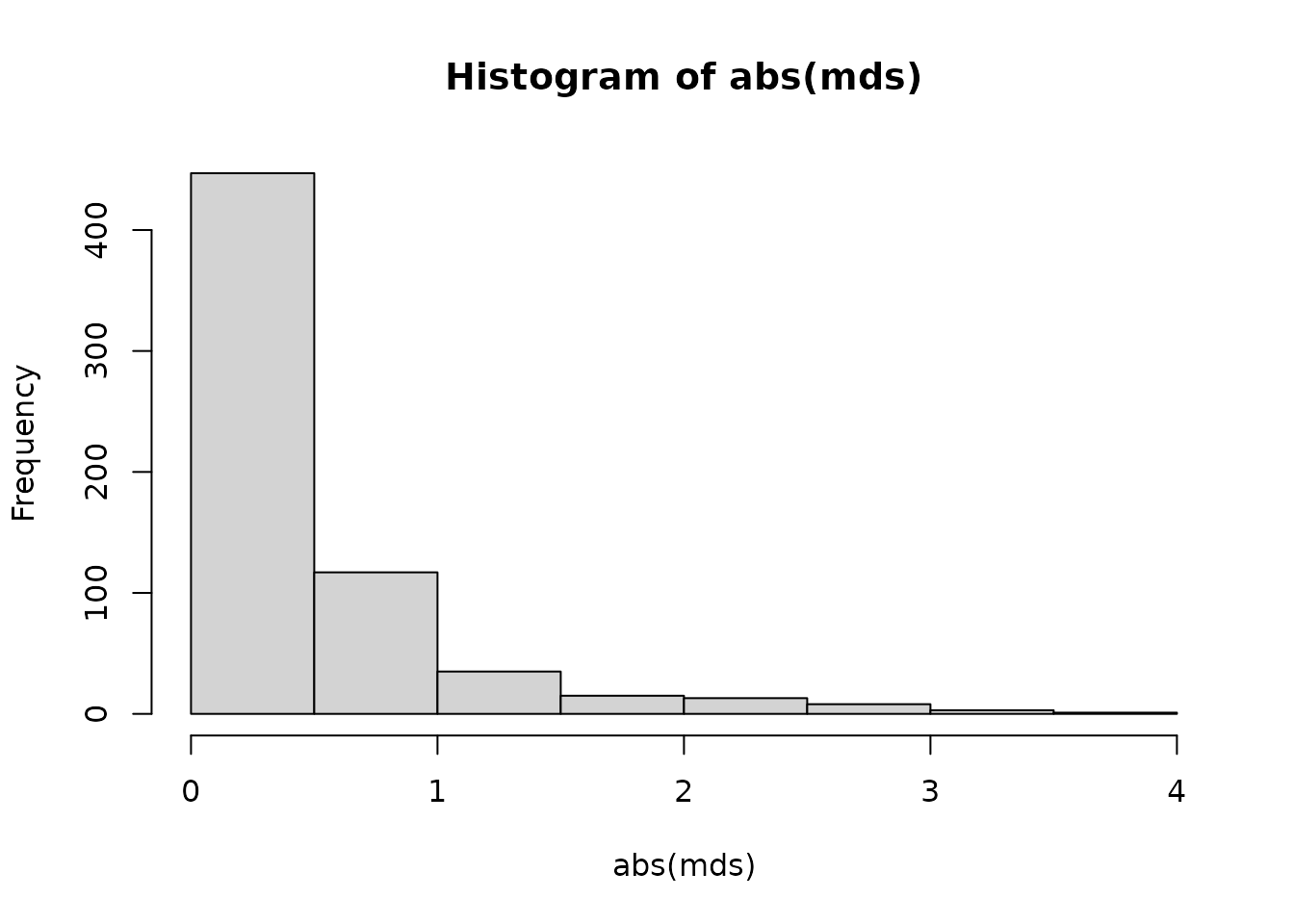
plot(stdErr, mds, frame.plot = FALSE, xlab = "Standard error of estimate",
     ylab = "Difference, stepping stone vs path sampling estimates",
     col = ModelCol(modelsN), pch = 16)
abline(h = 0, lty = "dashed", col = "grey70")
abline(0, 1, lty = "dashed", col = "grey70")
legend("topleft", ModelLabel(modelsN), pch = 16, col = ModelCol(modelsN),
       bty = "n")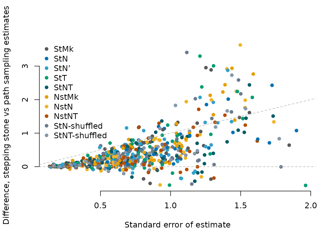
We compare models with and without a free n under both stationary and non-stationary assumptions, checking whether gains over the symmetric Mk model are replicated relative to randomised controls.
# Number in which StN outperforms StMk
.ErrCompare <- function(mod1, mod2, eps = epsBF) {
  .OutwithError(marginals[mod1, ] - marginals[mod2, ],
                .DiffErr(stdErr[mod1, ], stdErr[mod2, ]), eps)
}
stnWins <- .ErrCompare("by_n_ki", "by_ki")
message("outperforms StMk in ", sum(stnWins), " of ", dim(marginals)[[2]])
## outperforms StMk in 24 of 64
# ... and number in which StN outperforms StN-shuffled
stnBeatsRandom <- stnWins & .ErrCompare("by_n_ki", "rm_by_n_ki")
message(sum(stnBeatsRandom, na.rm = TRUE), " of these ",
        sum(stnWins & !is.na(stnBeatsRandom)))
## 17 of these 24
message(
  "StMk was preferred in ",
  # Number in which StMk outperforms StN
  sum(.ErrCompare("by_n_ki", "by_ki")),
  " of ", # Number of datasets for which data are available
  sum(!is.na(marginals["by_n_ki", ] < marginals["by_ki", ])),
  " datasets.")
## StMk was preferred in 24 of 64 datasets.
stNt <- .ErrCompare("by_nt_ki", "by_t_ki")
message(
  "StNT outperforms StT in ", sum(stNt), "/", sum(!is.na(stNt)),
  " datasets, and underperforms in ",
  sum(.ErrCompare("by_t_ki", "by_nt_ki")))
## StNT outperforms StT in 26/64 datasets, and underperforms in 3
stnWithT <- .ErrCompare("by_nt_ki", "by_t_ki") & .ErrCompare("by_t_ki", "by_ki")
message("StNT beats StT in ", sum(stnWithT), " of ",
        sum(.ErrCompare("by_t_ki", "by_ki")),
        " cases where free t param is supported")
## StNT beats StT in 8 of 15 cases where free t param is supported
EvaluateMk2 <- function(marginals, stdErr, epsBF = 1, suffix = "_ki") {

  models <- c("by", "by_n", "by_t", "by_nt") |> paste0(suffix) |>
    setNames(c("base", "n", "t", "nt"))
  mk2 <- ModelBF(marginals, models)
  baseMarginal <- marginals[models[c("base", "t")], ]
  colSelect <- !is.na(baseMarginal[1, ])
  baseRow <- apply(baseMarginal[, colSelect], 2, which.max)
  baseModel <- models[c("base", "t")[baseRow]]
  nModel <- models[c("n", "nt")[baseRow]]

  baseMarginal <- marginals[cbind(baseModel, names(baseRow))]
  nMarginal <- marginals[cbind(nModel, names(baseRow))]

  baseErr <- stdErr[cbind(baseModel, names(baseRow))]
  nErr <- stdErr[cbind(nModel, names(baseRow))]

  nImprovement <- nMarginal - baseMarginal

  good <- .OutwithError(nImprovement, .DiffErr(baseErr, nErr), epsBF)
  bad <- .OutwithError(-nImprovement, .DiffErr(baseErr, nErr), epsBF)
  ugly <- !good & !bad

  message("Mk2 improves in ", sum(good, na.rm = TRUE),
          ", indifferent in ", sum(ugly, na.rm = TRUE),
          "; deleterious in ", sum(bad, na.rm = TRUE), " / ",
          sum(!is.na(nImprovement)), " projects.")

  invisible(structure(
    nImprovement,
    names = names(baseRow),
    nBetter = good,
    nWorse = bad,
    err = nErr))
}

mk2 <- EvaluateMk2(marginals, stdErr, eps = epsBF)
## Mk2 improves in 25, indifferent in 33; deleterious in 6 / 64 projects.
betterNames <- names(mk2)[which(attr(mk2, "nBetter"))]
rm <- marginals[c("by_n_ki", "rm_by_n_ki"), betterNames]
rm <- rm[, colSums(is.na(rm)) == 0]
message(sum(rm[2, ] < rm[1, ]), " (",
        sum(.OutwithError(rm[2, ] - rm[1, ],
                          .DiffErr(stdErr["by_n_ki", colnames(rm)],
                                   stdErr["rm_by_n_ki", colnames(rm)]))),
        " by eps) / ", ncol(rm), " projects prefer by_n_ki to rm_by_n_ki")
## 22 (2 by eps) / 25 projects prefer by_n_ki to rm_by_n_ki
# Equivalent numbers under non-stationary model
# Number in which NstN outperforms NstMk
nstnWins <- .ErrCompare("ns_n_ki", "ns_ki")
length(which(nstnWins))
## [1] 27## [1] 64## [1] 0
# Number of datasets for which data are available
sum(!is.na(marginals["ns_n_ki", ] < marginals["ns_ki", ]))
## [1] 64
# Summary: very similar, with slightly more preferring free nWe visualise Mk2 model support as a function of dataset composition (neo:trans ratio, character count, taxon count) and by taxonomic group.
mk2Col <- hcl.colors(6, "Red-Green")[c(2, 2, 5, 5)][
  cut(mk2, breaks = c(-Inf, -epsBF, 0, epsBF, Inf))]

plot(.meta$nChar["neo", names(mk2)] / .meta$nChar["trans", names(mk2)], mk2,
     log = "x", col = mk2Col, pch = 3,
     frame.plot = FALSE, xlab = "Neo:Trans", ylab = "Mk2 BF")
EpsLine()
abline(v = 1)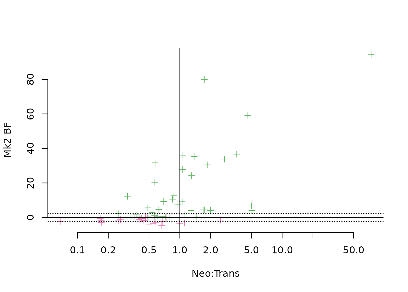
plot(colSums(.meta$nChar[, names(mk2)]), mk2,
     log = "x", col = mk2Col, pch = 3,
     frame.plot = FALSE, xlab = "Number of characters", ylab = "Mk2 BF")
EpsLine()
abline(v = 1)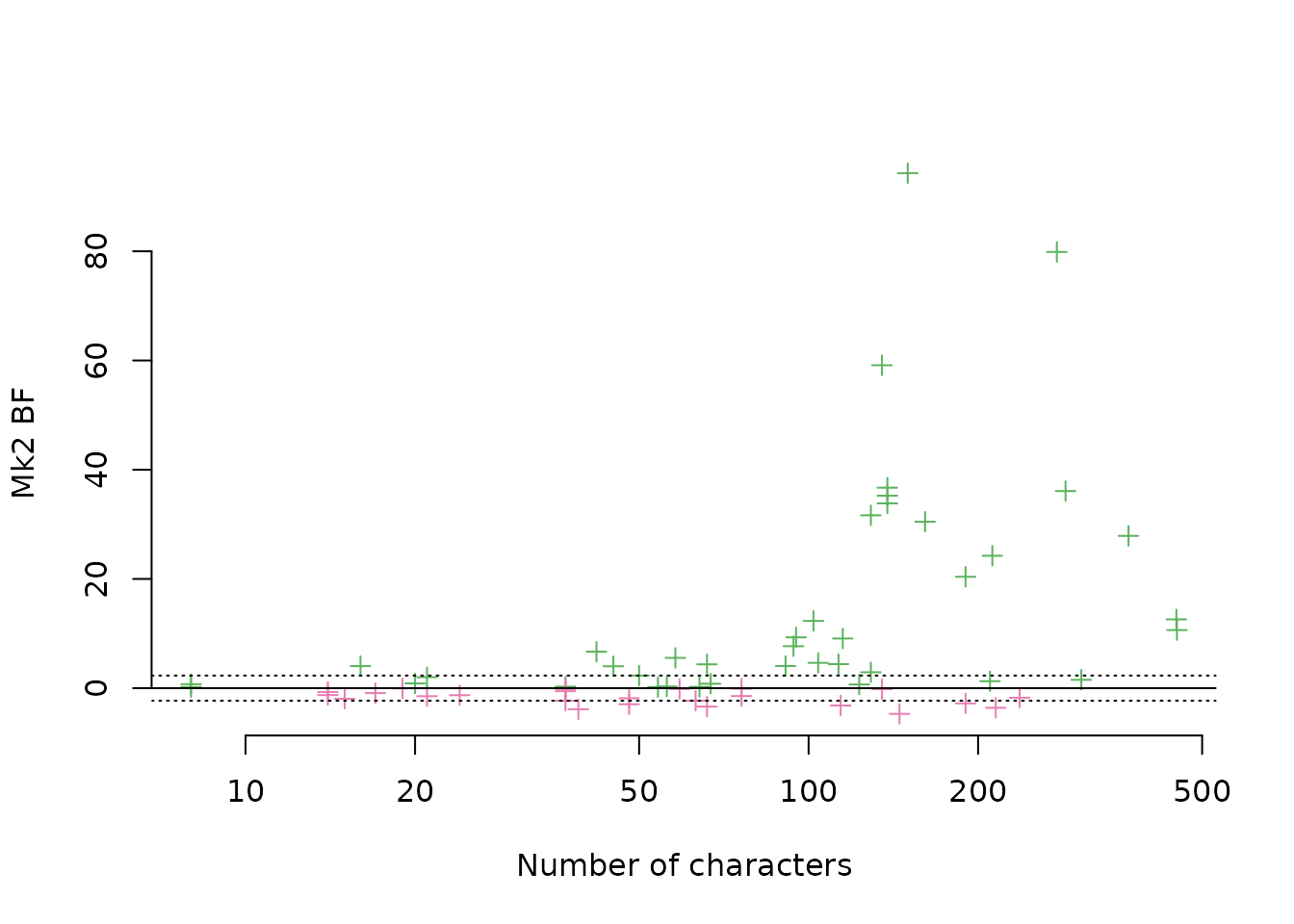
plot(.meta$nTaxa[names(mk2)], mk2,
     log = "x", col = mk2Col, pch = 3,
     frame.plot = FALSE, xlab = "Number of taxa", ylab = "Mk2 BF")
EpsLine()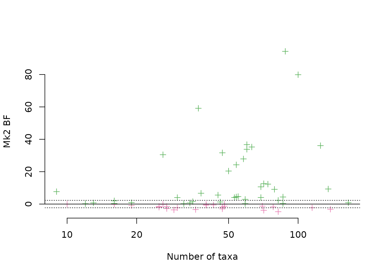
For completeness, we evaluate whether non-stationary Mk and Mk2 models improve on each other and on their stationary counterparts.
EvaluateNonStat <- function(marginals, se, epsBF = 1, suffix = "_ki") {

  models <- c("by", "by_n", "ns", "ns_n") |> paste0(suffix) |>
    setNames(c("s", "sn", "ns", "nsn"))
  ml <- ModelBF(marginals, models)

  ns_helps <- .OutwithError(ml[models[["ns"]], ] - ml[models[["s"]], ],
                            .DiffErr(se[models[["ns"]], ], se[models[["s"]], ]),
                            epsBF)
  ns_hinders <- .OutwithError(ml[models[["s"]], ] - ml[models[["ns"]], ],
                              .DiffErr(se[models[["ns"]], ], se[models[["s"]], ]),
                              epsBF)
  mk2_helps <- .OutwithError(ml[models[["sn"]], ] - ml[models[["s"]], ],
                             .DiffErr(se[models[["sn"]], ], se[models[["s"]], ]),
                             epsBF)
  mk2_hinders <- .OutwithError(ml[models[["s"]], ] - ml[models[["sn"]], ],
                               .DiffErr(se[models[["s"]], ], se[models[["sn"]], ]),
                               epsBF)
  both_beat_ns <- ns_helps & .OutwithError(
    ml[models[["nsn"]], ] - ml[models[["ns"]], ],
    .DiffErr(se[models[["nsn"]], ], se[models[["ns"]], ]),
    epsBF)
  both_beat_mk2 <- mk2_helps & .OutwithError(
    ml[models[["nsn"]], ] - ml[models[["sn"]], ],
    .DiffErr(se[models[["nsn"]], ], se[models[["sn"]], ]),
    epsBF)

  message("Non-stat improves in ", sum(ns_helps), "/", ncol(ml),
          " (worse in ", sum(ns_hinders),
          "), of which Mk2 further improves ", sum(both_beat_ns), ".")
  message("Mk2 improves in ", sum(mk2_helps), "/", ncol(ml),
          " (worse in ", sum(mk2_hinders),
          "), of which Non-stat further improves ", sum(both_beat_mk2), ".")

  invisible(ml)
}

EvaluateNonStat(marginals, stdErr, eps = epsBF)
## Non-stat improves in 15/64 (worse in 3), of which Mk2 further improves 9.## Mk2 improves in 24/64 (worse in 4), of which Non-stat further improves 5.
ns <- marginals["ns_ki", ] - marginals["by_ki", ]
ns_n <- marginals["ns_n_ki", ] - marginals["by_ki", ]
by_n <- marginals["by_n_ki", ] - marginals["by_ki", ]
plot(ns ~ by_n, asp = 1, frame.plot = FALSE)
EpsLine(diag = TRUE)
plot(ns_n ~ by_n, asp = 1, frame.plot = FALSE,
     xlab = "Mkn - Mk", ylab = "ns_n - Mk")
EpsLine(vert = TRUE, diag = TRUE)
plot(marginals["ns_n_ki", ] - marginals["ns_ki", ],
     marginals["by_n_ki", ] - marginals["by_ki", ],
     xlab = "+n, non-stat", ylab = "+n, stationary",
     asp = 1, frame.plot = FALSE)
EpsLine(vert = TRUE, diag = TRUE)
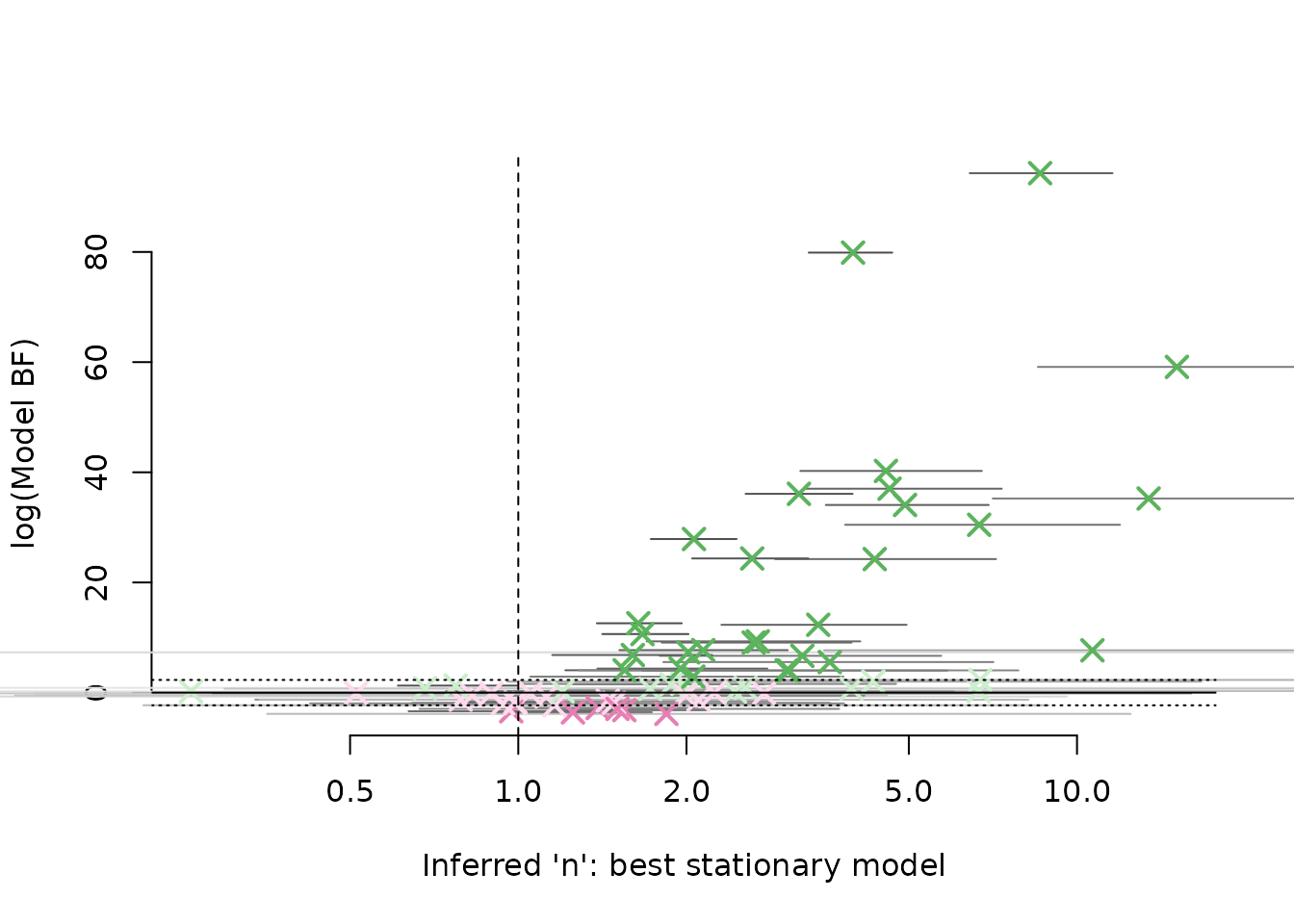
We extract the posterior distribution of n under the best-fitting stationary model for each dataset, and test whether inferred values differ significantly from one.
# Compare estimated values of n
bestNModel <- ifelse(marginals["by_n_ki", ] > marginals["by_nt_ki", ],
                     "by_n_ki", "by_nt_ki")
nProjects <- names(bestNModel)[!is.na(bestNModel)]

# Estimated value of n using the best available stationary model
# Strictly, this vector stores 1 / n, i.e. rate_loss not rate_gain
stationaryN <- sapply(nProjects, function(pID) {
  res <- ExistingResults(pID, bestNModel[pID],
                  checkRemote = FALSE)[["parameters"]][, "rate_loss"]
  if (is.null(res)) {
    message("Need results for ", pID, "_", bestNModel[pID])
    RevBayes(pID, bestNModel[pID])
    MakeSlurm(pID, bestNModel[pID], ml = FALSE)
  }
  res %||% setNames(rep(NA, 6), c("2.5%", "25%", "50%", "75%", "97.5%", "mad"))
})

nNotOne <- stationaryN["97.5%", ] < 1 | stationaryN["2.5%", ] > 1
# convert 1 / rate_loss yields rate_gain
n50 <- 1 / stationaryN["50%", ]
exp(summary(log(n50)))
## Min. 1st Qu. Median Mean 3rd Qu. Max.
## 0.06625 0.30510 0.49713 0.46558 0.73958 3.85226
# vioplot::vioplot(log(t50), log(n50),
#                  names = c("log(t)", "log(n)"),
#                  frame.plot = FALSE)
shapiro.test(log(n50))
##
## Shapiro-Wilk normality test
##
## data: log(n50)
## W = 0.98515, p-value = 0.6373##
## One Sample t-test
##
## data: log(n50)
## t = -7.919, df = 63, p-value = 4.945e-11
## alternative hypothesis: true mean is not equal to 0
## 95 percent confidence interval:
## -0.9573925 -0.5715624
## sample estimates:
## mean of x
## -0.7644774## [1] 0.772301
message(
  "LogMean: ", signif(exp(mean(log(n50), na.rm = TRUE)), 3),
  ", sd ", paste0(signif(exp(mean(log(n50)) + c(-1, 1) * sd(log(n50), na.rm = TRUE)), 3), collapse = ", "),
  "; Median: ", signif(median(n50, na.rm = TRUE), 3),
  ", mad ", signif(mad(n50, na.rm = TRUE), 3)
)
## LogMean: 0.466, sd 0.215, 1.01; Median: 0.497, mad 0.316
message("Different from 1: ", sum(nNotOne, na.rm = TRUE),
        " / ", sum(!is.na(nNotOne)), ": ",
        sum(1 / stationaryN["97.5%", ] > 1, na.rm = TRUE), " > 1; ",
        sum(1 / stationaryN["2.5%", ] < 1, na.rm = TRUE), " < 1")
## Different from 1: 37 / 64: 2 > 1; 35 < 1
ntBest <- (bestNModel == "by_nt_ki")[!is.na(bestNModel)]
nModelBF <- setNames(numeric(length(nProjects)), nProjects)
nModelBF[ntBest] <- marginals["by_nt_ki", nProjects[ntBest]] -
  marginals["by_t_ki", nProjects[ntBest]]
nModelBF[!ntBest] <- marginals["by_n_ki", nProjects[!ntBest]] -
  marginals["by_ki", nProjects[!ntBest]]
nCol <- hcl.colors(6, "Red-Green")[2:5][
  cut(nModelBF, breaks = c(-Inf, -epsBF, 0, epsBF, Inf))]

{
  par(mfrow = c(1, 1))
  plot(stationaryN["50%", ], nModelBF,
       xlab = "Inferred 'n': best stationary model",
       ylab = "log(Model BF)", xpd = NA,
       frame.plot = FALSE, pch = 4, log = "x")
  confidenceCol <- gray.colors(256)
  iqr <- log(stationaryN["75%", ]) - log(stationaryN["25%", ])
  segments(stationaryN["2.5%", ], nModelBF, stationaryN["97.5%", ], xpd = NA,
           col = confidenceCol[cut(iqr, breaks = 256)])
  points(stationaryN["50%", ], nModelBF, col = nCol,
         pch = 4, cex = 1.5, lwd = 2)
  abline(v = 1, lty = 2)
  EpsLine()
}
For datasets where non-stationary models are preferred, we extract joint estimates of n and the root-state frequency a0, and check whether the two parameters are correlated.
bestNSNModel <- ifelse(marginals["ns_n_ki", ] > marginals["ns_nt_ki", ],
                       "ns_n_ki", "ns_nt_ki")
nsPreferred <- pmax(marginals["ns_n_ki", ], marginals["ns_nt_ki", ]) >
  pmax(marginals["by_n_ki", ], marginals["by_nt_ki", ])
nsPreferredEps <- pmax(marginals["ns_n_ki", ], marginals["ns_nt_ki", ]) >
  pmax(marginals["by_n_ki", ], marginals["by_nt_ki", ]) + epsBF
nsnProjects <- names(bestNSNModel)[!is.na(bestNSNModel)]

# Estimated value of 1/n and a0 using the best available non-stationary model
nsnCols <- c("root_freqs.1.", "rate_loss")
nsnRet <- matrix(NA_real_, 6, 2, dimnames = list(
  c("2.5%", "25%", "50%", "75%", "97.5%", "mad"), nsnCols))
nsnParams <- vapply(nsnProjects, function(pID) {
  params <- ExistingResults(pID, bestNSNModel[[pID]],
                            checkRemote = FALSE)[["parameters"]]
  if (is.null(params)) {
    message("Need results for ", pID, "_", bestNSNModel[pID])
    MakeSlurm(pID, bestNSNModel[[pID]], ml = FALSE)
  }
  params[, nsnCols] %||% nsnRet
}, nsnRet)
nsN <- 1 / nsnParams["50%", "rate_loss", ]
ns25 <- 1 / nsnParams["25%", "rate_loss", ]
ns75 <- 1 / nsnParams["75%", "rate_loss", ]

nsA0 <- nsnParams["50%", "root_freqs.1.", ]
plot(1 / (1 + nsN), nsA0, frame.plot = FALSE,
     xlab = "% absent at stationary distribution", ylab = "% absent at root",
     asp = 1, col = 1 + nsPreferred[nsnProjects] + nsPreferredEps[nsnProjects])
segments(1 / (1 + nsN), nsnParams["25%", "root_freqs.1.", ],
         1 / (1 + nsN), nsnParams["75%", "root_freqs.1.", ],
         col = 1 + nsPreferred[nsnProjects] + nsPreferredEps[nsnProjects])
segments(1 / (1 + ns25), nsA0, 1 / (1 + ns75),
         col = 1 + nsPreferred[nsnProjects] + nsPreferredEps[nsnProjects])
abline(0, 1, lty = "dashed", col = 4)
legend("bottomleft", pch = 3, col = 1:3, bty = "n",
       legend = c("Stat pref.", "NS pref, < eps", "Non-Stat pref, > eps"))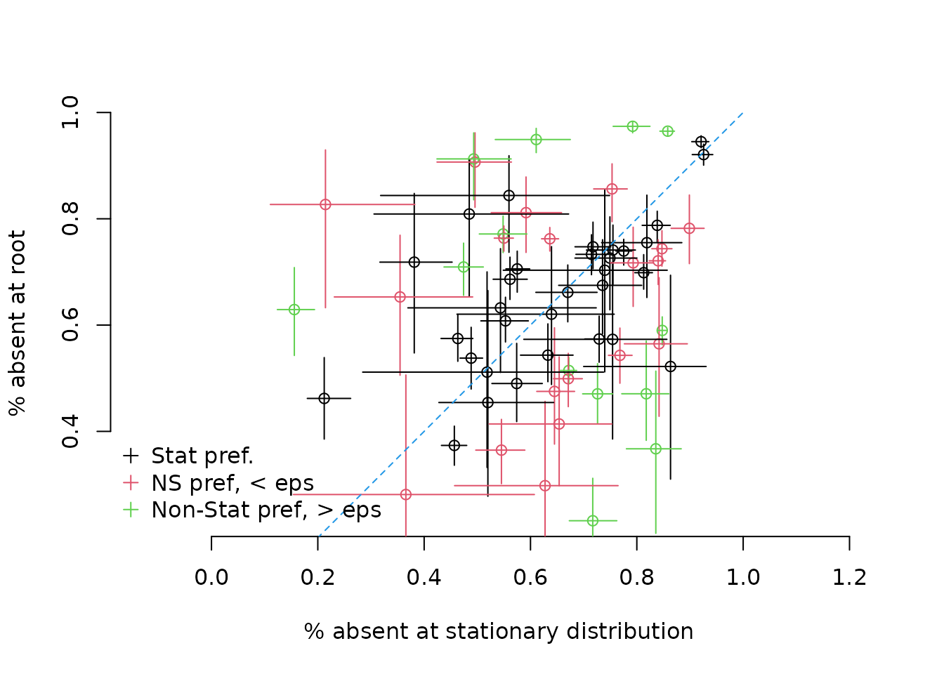
plot(nsA0, frame.plot = FALSE)
Variable-selection random forests identify metadata predictors of Mk2 model support and of the inferred value of n.
# Which variables predict support for a model with a free n?
nProj <- names(nModelBF)
meta <- data.frame(
  nModelBF,
  nChar = colSums(.meta$nChar[, nProj]),
  nTrans = .meta$nChar["trans", nProj],
  nNeo = .meta$nChar["neo", nProj],
  logNTRatio = log(.meta$nChar["neo", nProj] / .meta$nChar["trans", nProj]),
  charPerTax = colSums(.meta$nChar[, nProj]) / .meta$nTaxa[nProj],
  taxon = .meta$taxon[nProj],
  rank = .meta$rank[nProj],
  nTaxa = .meta$nTaxa[nProj],
  inferredN = t(stationaryN[, nProj])
)

nPredictors <- c("nChar", "logNTRatio", "charPerTax", "taxon", "rank", "nTaxa",
                 "inferredN.50.")
vsurfBF <- VSURF::VSURF(meta[, nPredictors], nModelBF, verbose = FALSE)

predBF <- nPredictors[vsurfBF[["varselect.interp"]]]
cat(paste0(predBF, collapse = ", "))
## inferredN.50., nChar, logNTRatio
rfBF <- randomForest(meta[, predBF, drop = FALSE], nModelBF,
                     ntree = 10000, importance = TRUE)
importance(rfBF)
## %IncMSE IncNodePurity
## inferredN.50. 83.24828 7709.228
## nChar 90.83067 6307.041
## logNTRatio 52.33797 7325.937
varImpPlot(rfBF, frame.plot = FALSE)
nPred <- length(predBF)

par(mfrow = c(nPred, 2))
for (predictor in predBF) {
  partialPlot(rfBF, meta[, nPredictors], as.character(predictor),
              frame.plot = FALSE, xlab = as.character(predictor))
  plot(nModelBF ~ meta[, predictor], frame.plot = FALSE, xlab = predictor)
  EpsLine()
}
metaN <- meta[!is.na(meta[, "inferredN.50."]), ]
n50 <- metaN[, "inferredN.50."]
vsurfN <- VSURF::VSURF(metaN[, nPredictors], log(n50), verbose = FALSE)
predN <- nPredictors[vsurfN[["varselect.interp"]]]

message(paste(predN, collapse = ", "))
## inferredN.50.
# Expect this to be zero, or perhaps higher taxon
rfT <- randomForest(metaT[, tPredictors[vsurfT[["varselect.pred"]]]],
                    t50,
                    ntree = 10000, importance = TRUE)

varImpPlot(rfT, frame.plot = FALSE)
par(mfrow = c(2, 1))
partialPlot(rfT, metaT, logNTRatio)
plot(t50 ~ metaT$logNTRatio, frame.plot = FALSE, log = "y")
## Warning in xy.coords(x, y, xlabel, ylabel, log): 8 y values <= 0 omitted from
## logarithmic plot
abline(h = 1, lty = "dotted")
partialPlot(rfT, metaT, nTaxa)
plot(t50 ~ metaT$nTaxa, frame.plot = FALSE, log = "y")
## Warning in xy.coords(x, y, xlabel, ylabel, log): 8 y values <= 0 omitted from
## logarithmic plot
abline(h = 1, lty = "dotted")
par(mfrow = c(1, 1))
plot(.meta$nChar["trans", ], .meta$nChar["neo", ],
     pch = ifelse(abs(mk2) > epsBF, 16, 1),
     col = mk2Col,
     xlab = "Transformational characters", ylab = "Neomorphic characters",
     log = "xy",
     asp = 1, frame.plot = FALSE)
abline(0, 1, lty = "dashed")
legend("topleft", bty = "n",
       legend = c("mk2 preferred", "> eps", "<= eps",  "mk preferred"),
       pch = c(16, 1, 1, 16), pt.cex = 1.2,
       col = hcl.colors(6, "Red-Green")[c(5, 5, 2, 2)])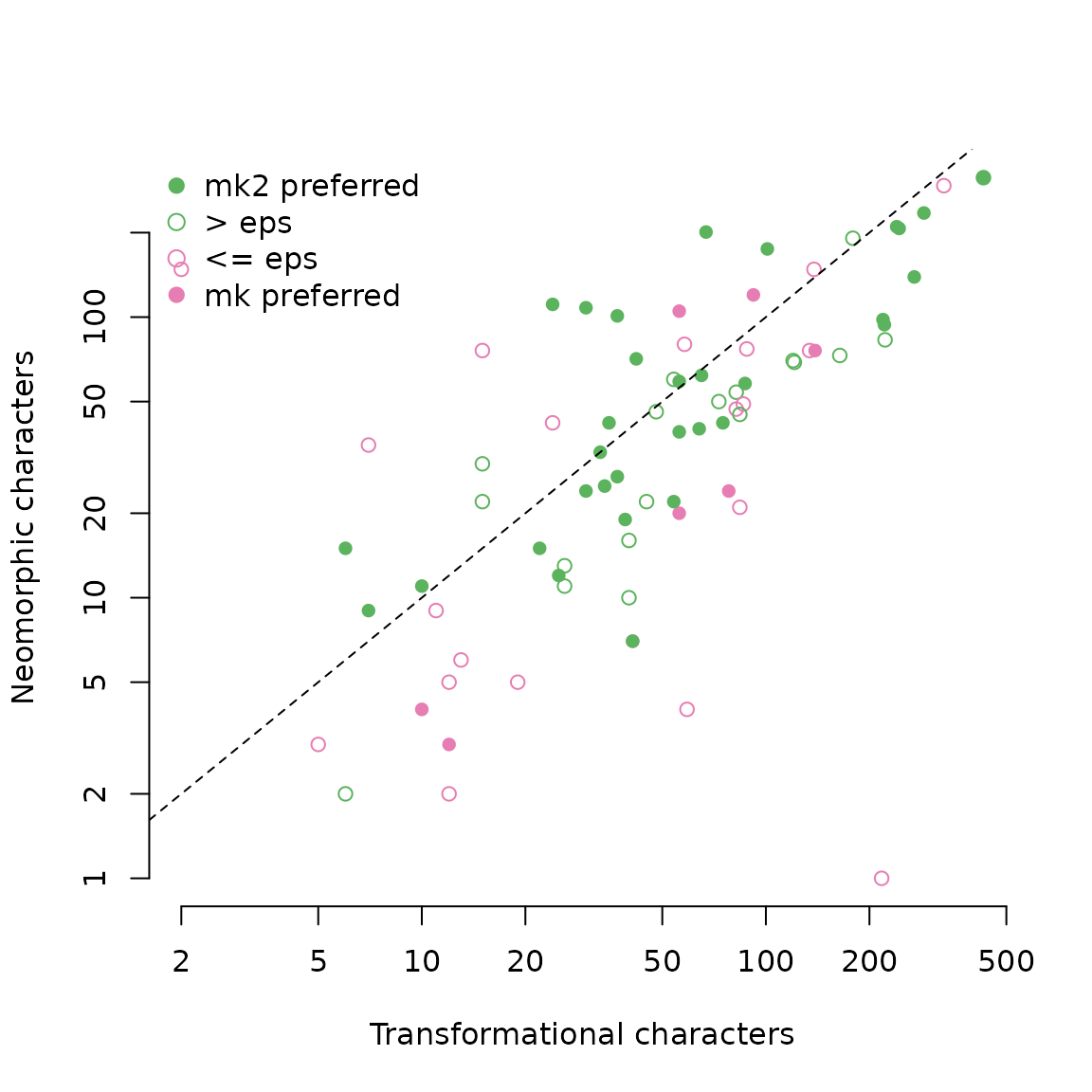
plot(colSums(.meta$nChar), .meta$nTaxa,
     pch = ifelse(abs(mk2) > epsBF, 16, 1),
     col = mk2Col,
     xlab = "Characters", ylab = "Taxa",
     log = "xy", frame.plot = FALSE)
abline(0, 1, type = "dashed")
## Warning in int_abline(a = a, b = b, h = h, v = v, untf = untf, ...): graphical
## parameter "type" is obsolete
legend("topleft", bty = "n",
       legend = c("mk preferred", "<eps", "<eps", "mk2 preferred"),
       pch = c(16, 1, 1, 16), pt.cex = 1.2,
       col = hcl.colors(6, "Red-Green")[2:5])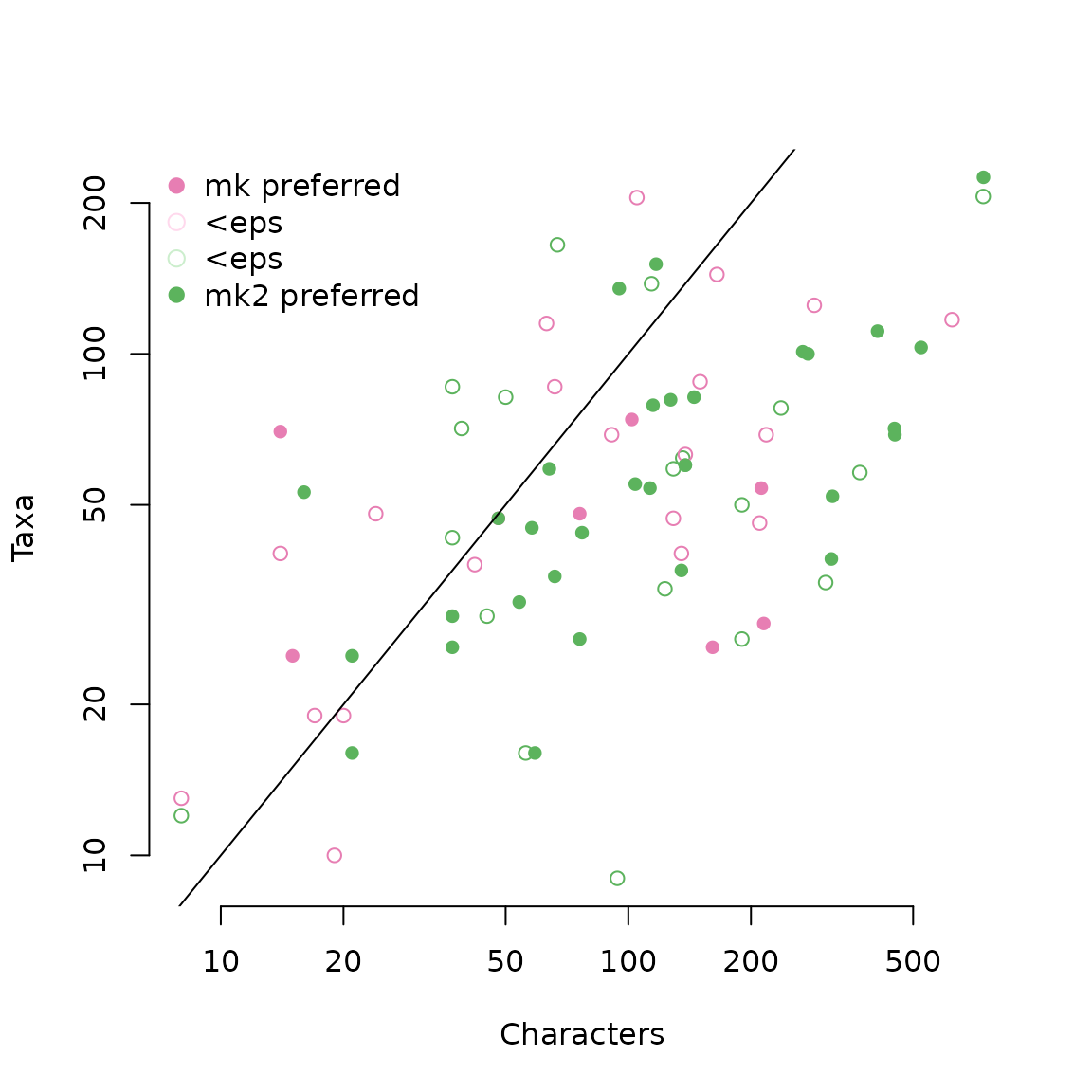
boxplot(mk2 ~ .meta$taxon[names(mk2)], las = 2,
        frame.plot = FALSE, cex = 0.8, ylab = "MK2 BF", notch = TRUE,
        col = TaxonCol())
## Warning in (function (z, notch = FALSE, width = NULL, varwidth = FALSE, : some
## notches went outside hinges ('box'): maybe set notch=FALSE
EpsLine()
SpindleCompare("by_nn_ki", "by_n_ki", marginals, stdErr)## better worse n
## by_nn_ki 8 8 64
abline(h = 0, lty = 2, lwd = 1, col = "grey70")
nnWins <- .OutwithError(marginals["by_nn_ki", ] -
                          marginals["by_n_ki", ],
                        stdErr["by_nn_ki", ], stdErr["by_n_ki", ])
nWins <- .OutwithError(marginals["by_n_ki", ] -
                         marginals["by_nn_ki", ],
                       stdErr["by_nn_ki", ], stdErr["by_n_ki", ])

sum(nnWins)
## [1] 22
sum(nWins)## [1] 17
.OutwithError(marginals["by_nt_ki", ] - marginals["by_n_ki", ],
              .DiffErr(stdErr["by_nt_ki", ], stdErr["by_n_ki", ])) |>
  sum() # Similar to by_t_ki vs by_ki
## [1] 20
.OutwithError(marginals["by_nt_ki", ] - marginals["by_nn_ki", ],
              .DiffErr(stdErr["by_nt_ki", ], stdErr["by_nn_ki", ]))
## 104 157 175 450 493 563 635 675 692 706 748 950 1113
## FALSE TRUE FALSE FALSE FALSE FALSE FALSE FALSE FALSE TRUE FALSE FALSE FALSE
## 1210 1271 2131 2553 2800 3199 3200 3244 3351 3392 3405 3408 3445
## FALSE FALSE FALSE TRUE TRUE FALSE FALSE TRUE FALSE FALSE FALSE TRUE TRUE
## 3448 3603 3646 3655 3705 3710 3711 3755 3757 3804 3832 3833 3927
## FALSE FALSE FALSE FALSE TRUE FALSE TRUE FALSE FALSE FALSE FALSE FALSE TRUE
## 3929 4111 4220 4230 4291 4305 4308 4309 4310 4467 4649 4747 4761
## FALSE FALSE FALSE FALSE FALSE FALSE FALSE TRUE FALSE FALSE TRUE FALSE TRUE
## 4790 4867 4910 5099 5186 5201 5228 5230 5255 5268 5327 07203
## FALSE TRUE TRUE FALSE FALSE FALSE TRUE FALSE FALSE TRUE FALSE FALSE
.OutwithError(marginals["by_nn_ki", ] - marginals["by_n_ki", ],
              .DiffErr(stdErr["by_nn_ki", ], stdErr["by_n_ki", ])) |>
  sum()
## [1] 8
.OutwithError(marginals["by_n_ki", ] - marginals["by_nn_ki", ],
              .DiffErr(stdErr["by_nn_ki", ], stdErr["by_n_ki", ])) |>
  sum()
## [1] 8
plot(marginals["by_nn_ki", ] - marginals["by_n_ki", ] ~
       I(2 * stdErr["by_nn_ki", ]), frame = 0); abline(h = 0, lty = 2); abline(0, 1, lty = 3); abline(0, -1, lty = 3)
plot(marginals["by_nn_ki", ] - marginals["by_ki", ],
     marginals["by_nn_ki", ] - marginals["by_n_ki", ],
     frame = 0,
     col = ModelCol("by_nn_ki"), pch = 16,
     xlim = range(t(marginals) - marginals["by_ki", ], na.rm = TRUE),
     xlab = "Advantage over StMk")
abline(h = 0)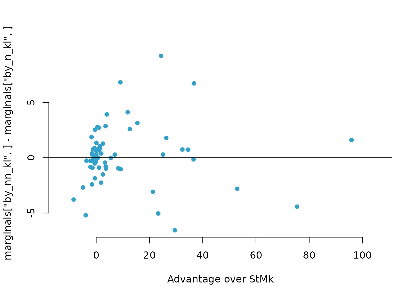
rate01 <- vapply(KiProjects(), function(pID) {
  x <- ExistingResults(pID, "by_nn_ki")[["parameters"]]
  if (is.null(x)) {
    rep(NA_real_, 6)
  } else {
    x[, "rate01"]
  }
}, ExistingResults(450, "by_nn_ki")[["parameters"]][, "rate01"])
medN <- rate01["50%", ]
hist(log(medN))
abline(v = 0, lwd = 3)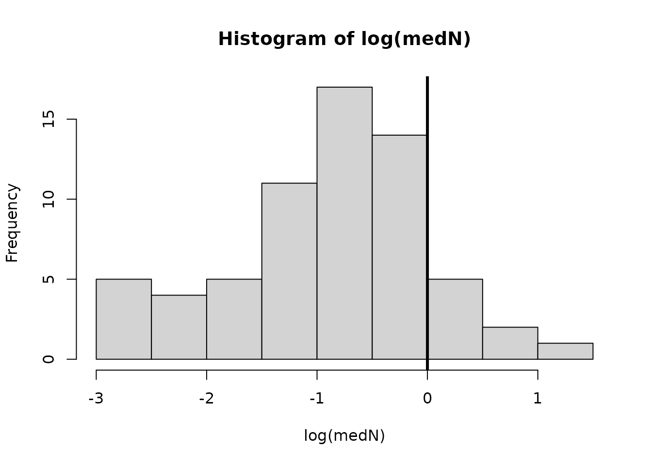
1 / median(medN, na.rm = TRUE)## [1] 2.422601
shapiro.test(log(medN))##
## Shapiro-Wilk normality test
##
## data: log(medN)
## W = 0.97302, p-value = 0.1734## Min. 1st Qu. Median Mean 3rd Qu. Max.
## -2.910 -1.420 -0.885 -0.929 -0.380 1.070## [1] 0.88## [1] 0.768##
## One Sample t-test
##
## data: log(medN)
## t = -8.4402, df = 63, p-value = 6.076e-12
## alternative hypothesis: true mean is not equal to 0
## 95 percent confidence interval:
## -1.1487409 -0.7089143
## sample estimates:
## mean of x
## -0.9288276
#sum(rate01["97.5%", ] < 1, na.rm = TRUE)
message("_n_ differs from unity (w/ pp > 95%) in ",
        sum(rate01["97.5%", ] < 1 | rate01["2.5%", ] > 1, na.rm = TRUE),
        " of ", sum(!is.na(medN)),
        " datasets, and is less than one in ",
        sum(rate01["97.5%", ] < 1, na.rm = TRUE),
        " of these")
## _n_ differs from unity (w/ pp > 95%) in 41 of 64 datasets, and is less than one in 39 of theseNon-stationarity
Non-stationary models allow the root-state frequency to differ from the stationary distribution implied by the gain and loss rates, with the departure parameterised by a0. As before, marginal likelihood estimates are first validated.
modelsNS <- c("by_ki", "by_n_ki", "by_nt_ki",
              "ns_ki", "ns_n_ki", "ns_nt_ki")
marginals <- GetMarginals(KiProjects(), modelsNS)
stdErr <- attr(marginals, "stdErr")
mds <- MarginalDiffs(KiProjects(), modelsNS)
hist(abs(mds), breaks = ceiling(max(abs(mds), na.rm = TRUE) * 2), xpd = NA)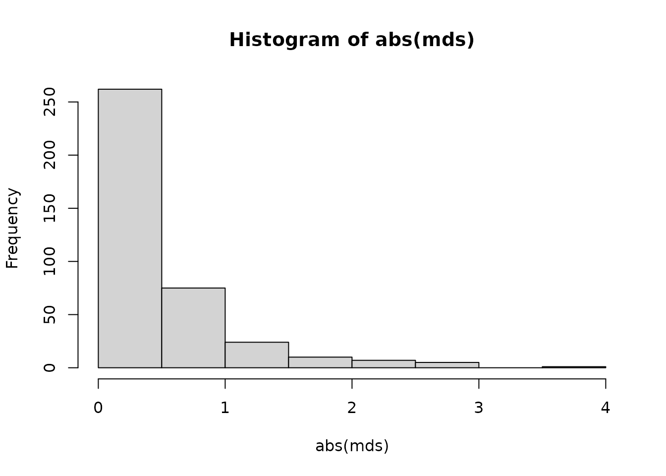
plot(stdErr, mds, frame.plot = FALSE, xlab = "Standard error of estimate",
     ylab = "Difference, stepping stone vs path sampling estimates",
     col = ModelCol(modelsNS), pch = 16)
abline(h = 0, lty = "dashed", col = "grey70")
abline(0, 1, lty = "dashed", col = "grey70")
legend("topleft", ModelLabel(modelsNS), pch = 16, col = ModelCol(modelsNS),
       bty = "n")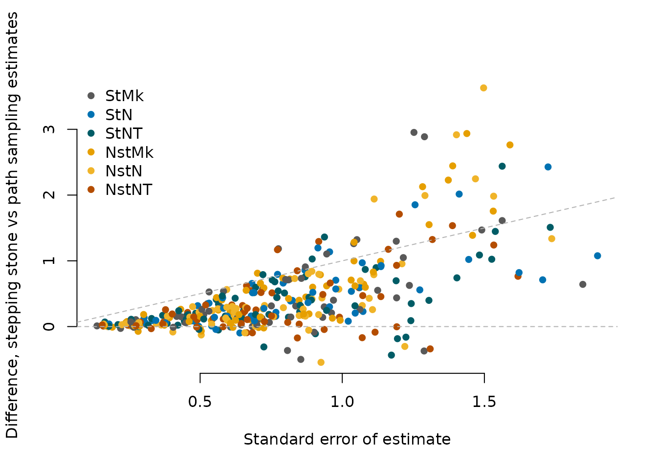
We determine how often the best non-stationary model outperforms the best stationary model, and vice versa.
StatCompare <- function(suffix) {
  ns <- paste0("ns_", suffix)
  st <- paste0("by_", suffix)
  paste0(ModelLabel(ns), " outperforms (underperforms) ", ModelLabel(st),
         " in ", sum(.ErrCompare(ns, st)), " (",
         sum(.ErrCompare(st, ns)), ") datasets"
  )
}
bestS <- apply(marginals[1:3, ], 2, which.max)
bestNS <- apply(marginals[4:6, ], 2, which.max)

bestML_S  <- marginals[cbind(bestS,  seq_len(ncol(marginals)))]
bestML_NS <- marginals[cbind(3 + bestNS, seq_len(ncol(marginals)))]

bestSE_S  <- stdErr[cbind(bestS,  seq_len(ncol(stdErr)))]
bestSE_NS <- stdErr[cbind(3 + bestNS, seq_len(ncol(stdErr)))]

paste(
  "the best-fitting non-stationary model outperforms the best stationary",
  "model in",
  sum(.OutwithError(bestML_NS - bestML_S, .DiffErr(bestSE_S, bestSE_NS))),
  "of", sum(!is.na(bestML_NS - bestML_S)),
  "datasets, and is outperformed in",
  sum(.OutwithError(bestML_S - bestML_NS, .DiffErr(bestSE_S, bestSE_NS)))
)
## [1] "the best-fitting non-stationary model outperforms the best stationary model in 11 of 64 datasets, and is outperformed in 6"
StatCompare("ki")## [1] "NstMk outperforms (underperforms) StMk in 15 (3) datasets"
StatCompare("n_ki")## [1] "NstN outperforms (underperforms) StN in 10 (6) datasets"
StatCompare("nt_ki")## [1] "NstNT outperforms (underperforms) StNT in 13 (6) datasets"We extract the root-frequency parameter a0 from the best-fitting non-stationary model for each dataset.
# For which analyses are results available?
allIn <- colSums(is.na(marginals)) == 0
someIn <- colSums(!is.na(marginals[1:3, ])) > 0 &
  colSums(!is.na(marginals[4:6, ])) > 0

# Take parameter values from the best non-stationary and stationary models
nsPref <- `names<-`(bestML_NS - bestML_S, colnames(marginals))
nullParam <- c(`2.5%` = NA_real_, `25%` = NA_real_, `50%` = NA_real_,
               `75%` = NA_real_, `97.5%` = NA_real_, mad = NA_real_)

nsValue <- sapply(seq_along(bestS), function(i) {
  ExistingResults(names(bestNS)[i], modelsNS[3 + bestNS[i]]
                  )[["parameters"]][, "root_freqs.1."] %||% nullParam
})
colnames(nsValue) <- names(bestS)
We test whether the log-odds root frequency departs significantly from zero (i.e. from equal root-state probabilities).
# Is the median root frequency different from zero?
# For results that include also ns_t_ki, see 5_Parameters.R
# The values there (not here) are used for publication
ns50 <- nsValue["50%", ]
a0 <- nsValue / (1 - nsValue)
f01 <- log(a0["50%", ])
exp(summary(f01))
## Min. 1st Qu. Median Mean 3rd Qu. Max.
## 0.3019 1.0843 2.1305 2.1308 3.1540 37.4638
sd(f01, na.rm = TRUE)## [1] 0.9898556
mad(f01, na.rm = TRUE)## [1] 0.8427146
shapiro.test(f01)##
## Shapiro-Wilk normality test
##
## data: f01
## W = 0.95836, p-value = 0.03009
e1071::skewness(f01, na.rm = TRUE)## [1] 0.6833221
t.test(f01)##
## One Sample t-test
##
## data: f01
## t = 6.1141, df = 63, p-value = 6.784e-08
## alternative hypothesis: true mean is not equal to 0
## 95 percent confidence interval:
## 0.5092496 1.0037668
## sample estimates:
## mean of x
## 0.7565082
# Summary statistics for best model
a2.5 <- a0["2.5%", ]
a97.5 <- a0["97.5%", ]
sum(a2.5 > 1, na.rm = TRUE)
## [1] 25
sum(a97.5 < 1, na.rm = TRUE)## [1] 3
sum(a2.5 > 1 | a97.5 < 1, na.rm = TRUE)## [1] 28## [1] 64For robustness, we repeat using a single fixed model (NstMk) throughout rather than the best-fitting non-stationary model for each dataset.
# Repeat, using a single model throughout.  The results turn out to be similar.
# Take parameter values from NstMk
nsValue <- sapply(KiProjects(), function(pID) {
  ExistingResults(pID, "ns_ki"
                  )[["parameters"]][, "root_freqs.1."] %||% nullParam
})

ns2.5 <- nsValue["2.5%", ]
ns50 <- nsValue["50%", ]
ns97.5 <- nsValue["97.5%", ]
a2.5 <- log(ns2.5 / (1 - ns2.5))
a50 <- log(ns50 / (1 - ns50))
a97.5 <- log(ns97.5 / (1 - ns97.5))
sum(a2.5 > 1, na.rm = TRUE)
## [1] 5
sum(a97.5 < 1, na.rm = TRUE)## [1] 25
sum(a2.5 > 1 | a97.5 < 1, na.rm = TRUE)## [1] 30## [1] 64
1 / median(ns50, na.rm = TRUE)## [1] 1.614058
median(a50, na.rm = TRUE)## [1] 0.487682
# Take parameter values from NstN
nsnValue <- sapply(KiProjects(), function(pID) {
  ExistingResults(pID, "ns_n_ki"
                  )[["parameters"]][, "root_freqs.1."] %||% nullParam
})

nsn2.5 <- nsnValue["2.5%", ]
nsn50 <- nsnValue["50%", ]
nsn97.5 <- nsnValue["97.5%", ]
an2.5 <- log(nsn2.5 / (1 - nsn2.5))
an50 <- log(nsn50 / (1 - nsn50))
an97.5 <- log(nsn97.5 / (1 - nsn97.5))
sum(an2.5 > 1, na.rm = TRUE)
## [1] 5
sum(an97.5 < 1, na.rm = TRUE)## [1] 20
sum(an2.5 > 1 | an97.5 < 1, na.rm = TRUE)## [1] 25## [1] 64
1 / median(ns50, na.rm = TRUE)## [1] 1.614058
median(a50, na.rm = TRUE)## [1] 0.487682Variable-selection random forests identify metadata predictors of support for non-stationary models.
# Can we predict which projects will benefit from a non-stationary model?
nsProj <- intersect(names(nsPref), names(bestS)[!is.na(nsValue[1, ])])
nsMeta <- data.frame(
  nsProj = nsPref[nsProj],
  nChar = colSums(.meta$nChar[, nsProj]),
  nTrans = .meta$nChar["trans", nsProj],
  nNeo = .meta$nChar["neo", nsProj],
  logNTRatio = log(.meta$nChar["neo", nsProj] / .meta$nChar["trans", nsProj]),
  charPerTax = colSums(.meta$nChar[, nsProj]) / .meta$nTaxa[nsProj],
  rank = .meta$rank[nsProj],
  taxon = .meta$taxon[nsProj],
  nTaxa = .meta$nTaxa[nsProj],
  # nsValue = t(nsValue[, nsProj]), --> a0Value
  a0Value = nsValue["50%", nsProj] / (1 - nsValue["50%", nsProj])
)

nsPredictors <- c("nChar", "logNTRatio", "charPerTax", "rank",
                  "taxon", "nTaxa", "a0Value")
vsurfBF <- VSURF::VSURF(nsMeta[, nsPredictors], nsPref[nsProj], verbose = FALSE)
## Warning in VSURF_pred.default(x = x, y = y, ntree.pred = ntree.pred, err.interp = interp$err.interp, : Unable to perform prediction step, because the interpretation step
## did not eliminate variables## a0Value, charPerTax, logNTRatio
rfBF <- randomForest(nsMeta[, predBF, drop = FALSE], nsPref[nsProj],
                     ntree = 10000, importance = TRUE)
importance(rfBF)
## %IncMSE IncNodePurity
## a0Value 32.423864 323.9703
## charPerTax -1.339345 283.5464
## logNTRatio 14.684436 320.6024
varImpPlot(rfBF, frame.plot = FALSE)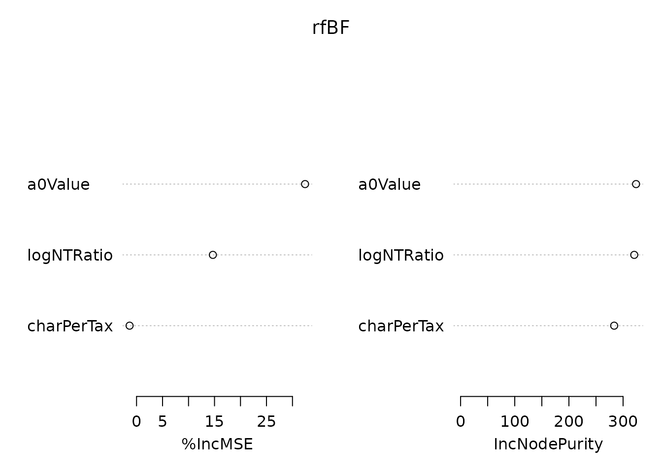
nPred <- length(predBF)

# Values of the root distribution that are uneven correspond to better support
# for non-stationary models.  This matches intuition.
# There is a prominent step where >250 characters suddenly give strong
# support for NS models.
par(mfrow = c(nPred, 2))
for (predictor in predBF) {
  partialPlot(rfBF, nsMeta[, nsPredictors], as.character(predictor))
  plot(nsPref[nsProj] ~ nsMeta[, predictor], frame.plot = FALSE, xlab = predictor)
  EpsLine()
}
Heterogeneous models
Heterogeneous models allow the 0↔︎1 rate to vary among characters, with variants differing in whether rate heterogeneity is shared across all two-state characters (Het1) or partitioned between neomorphic and transformational characters (Het, HetB, HetM, HetBM).
modelsHet <- c("by_ki", "by_n_ki", "by_nt_ki",
               "ns_ki", "ns_n_ki", "ns_nt_ki",
               "hg_ki", "hg2_ki", "hg_b_ki", "hg_m_ki", "hg_bm_ki")
marginals <- GetMarginals(KiProjects(), modelsHet)
stdErr <- attr(marginals, "stdErr")
mds <- MarginalDiffs(KiProjects(), modelsHet)
hist(abs(mds), breaks = ceiling(max(abs(mds), na.rm = TRUE) * 2), xpd = NA)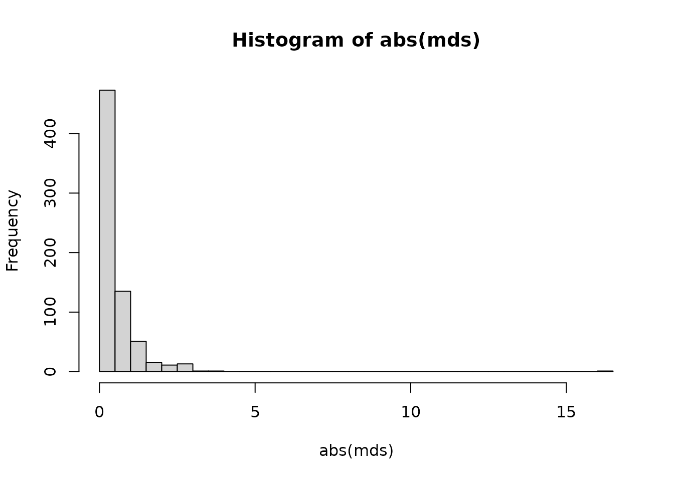
plot(stdErr, mds, frame.plot = FALSE, xlab = "Standard error of estimate",
     ylab = "Difference, stepping stone vs path sampling estimates",
     col = ModelCol(modelsHet), pch = 16)
abline(h = 0, lty = "dashed", col = "grey70")
abline(0, 1, lty = "dashed", col = "grey70")
legend("topleft", ModelLabel(modelsHet), pch = 16, col = ModelCol(modelsHet),
       bty = "N")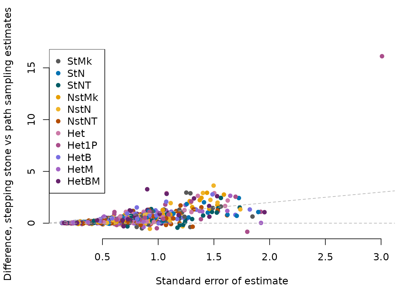
We identify datasets with complete results for both model families and select the best-fitting homogeneous and heterogeneous model for each.
# Which analyses are complete and have results available?
someIn <- colSums(!is.na(marginals[1:6, ])) > 0 &
  colSums(!is.na(marginals[6 + (1:5), ])) > 0
bestNH <- apply(marginals[1:6, someIn], 2, which.max)
bestHet <- apply(marginals[6 + (1:5), someIn], 2, which.max)
hetPref <- sapply(seq_along(bestHet), function(i) {
  marginals[6 + bestHet[[i]], someIn][[i]] - marginals[bestNH[i], someIn][[i]]
})
hetErr <- sapply(seq_along(bestHet), function(i) {
  .DiffErr(stdErr[6 + bestHet[[i]], someIn], stdErr[bestNH[i], someIn])[[i]]
})
We test whether the best heterogeneous model outperforms the best homogeneous model, and evaluate the added benefit of progressively finer partitioning of rate heterogeneity between neomorphic and transformational characters.
# Does the best het model beat the best homogeneous?
paste("The best heterogeneous gain–loss model outperforms its best homogeneous counterpart in",
      sum(.OutwithError(hetPref, hetErr, epsBF)),
      "of",
      length(hetPref),
      "datasets, whereas a homogeneous gain–loss model is preferred in",
      sum(.OutwithError(-hetPref, hetErr, epsBF)),
      "datasets.")
## [1] "The best heterogeneous gain–loss model outperforms its best homogeneous counterpart in 28 of 64 datasets, whereas a homogeneous gain–loss model is preferred in 14 datasets."
# Does allowing heterogeneity in transformational improve fit?
paste("Allowing 0↔1 heterogeneity across all two-state characters (model Het1)",
      "improves model fit relative to modelling 0↔1 heterogeneity only in",
      "neomorphic characters (model Het) in",
      sum(.ErrCompare("hg2_ki", "hg_ki"), na.rm = TRUE),            # 28
      "of",
      length(!is.na(marginals["hg2_ki", ] - marginals["hg_ki", ])), # 64
      "datasets and worsens it in",
      sum(.ErrCompare("hg_ki", "hg2_ki"), na.rm = TRUE)            # 4
)
## [1] "Allowing 0↔1 heterogeneity across all two-state characters (model Het1) improves model fit relative to modelling 0↔1 heterogeneity only in neomorphic characters (model Het) in 28 of 64 datasets and worsens it in 4"
# Does modelling distinct heterogeneity behaviour in Neo vs Trans improve fit?
hg2s <- c("hg_b_ki", "hg_m_ki", "hg_bm_ki")
# Which analyses have results available?
hgsIn <- colSums(is.na(marginals[c("hg2_ki", hg2s), ])) == 0

hbPref <- .ErrCompare("hg_b_ki", "hg2_ki")[hgsIn]
hmPref <- .ErrCompare("hg_m_ki", "hg2_ki")[hgsIn]
hbmPref <- .ErrCompare("hg_bm_ki", "hg2_ki")[hgsIn]
# Which of the bm models are best?
table(hg2s[apply(marginals[hg2s, hgsIn], 2, which.max)])
##
## hg_b_ki hg_bm_ki hg_m_ki
## 22 16 25
# How often does the best bm model outperform hg2?
hg2Pref <- hbPref | hmPref | hbmPref

# How often does hg2 outperform all bm models?
hbXPref <- .ErrCompare("hg2_ki", "hg_b_ki")[hgsIn]
hmXPref <- .ErrCompare("hg2_ki", "hg_m_ki")[hgsIn]
hbmXPref <- .ErrCompare("hg2_ki", "hg_bm_ki")[hgsIn]

paste(
  "Partitioning heterogeneity further by allowing distinct distributions of",
  "0↔1 rates for neomorphic and transformational partitions (using",
  "the best-fitting model of HetB, HetM and HetBM) offers only modest",
  "improvements, outperforming Het1 in",
  sum(hg2Pref),
  "of",
  sum(hgsIn),
  "datasets, and underperforming in",
  sum(hbXPref & hmXPref & hbmXPref)
)
## [1] "Partitioning heterogeneity further by allowing distinct distributions of 0↔1 rates for neomorphic and transformational partitions (using the best-fitting model of HetB, HetM and HetBM) offers only modest improvements, outperforming Het1 in 9 of 63 datasets, and underperforming in 3"
hg1Best <- sum(
  .ErrCompare("hg2_ki", "hg_b_ki")[hgsIn] &
  .ErrCompare("hg2_ki", "hg_m_ki")[hgsIn] &
  .ErrCompare("hg2_ki", "hg_bm_ki")[hgsIn]
)
sum(hg1Best)
## [1] 3
hg1Pref <- sum(
  .ErrCompare("hg2_ki", "hg_b_ki")[hgsIn] |
  .ErrCompare("hg2_ki", "hg_m_ki")[hgsIn] |
  .ErrCompare("hg2_ki", "hg_bm_ki")[hgsIn]
)
sum(hg1Pref)
## [1] 11
length(hg2Pref)## [1] 63Using a strict criterion (a model must outperform both competitors), we identify which of HetB, HetM and HetBM most consistently achieves the best fit.
ABestStrict <- function(a) {
  contenders <- setdiff(c("hg_b_ki", "hg_m_ki", "hg_bm_ki"), a)
  betterThanB <- .ErrCompare(a, contenders[[1]])[hgsIn]
  betterThanC <- .ErrCompare(a, contenders[[2]])[hgsIn]
  worseThanB <- .ErrCompare(contenders[[1]], a)[hgsIn]
  worseThanC <- .ErrCompare(contenders[[2]], a)[hgsIn]
  message(ModelLabel(a), " is best in ",
          sum(betterThanB & betterThanC),
          " and worst in ",
          sum(worseThanB & worseThanC)
  )
}

paste(
  "Differences among the fit of HetB, HetM and HetBM were negligible in",

  sum(!(.ErrCompare("hg_b_ki", "hg_m_ki") |
  .ErrCompare("hg_b_ki", "hg_bm_ki") |
  .ErrCompare("hg_m_ki", "hg_b_ki") |
  .ErrCompare("hg_m_ki", "hg_bm_ki") |
  .ErrCompare("hg_bm_ki", "hg_m_ki") |
  .ErrCompare("hg_bm_ki", "hg_b_ki"))[hgsIn]),
  "of",
  sum(hgsIn),
  "datasets"
)
## [1] "Differences among the fit of HetB, HetM and HetBM were negligible in 48 of 63 datasets"
message("in the remainder, ",
        "XXX performed better (worse) than both other models in..:")
## in the remainder, XXX performed better (worse) than both other models in..:
ABestStrict("hg_b_ki")## HetB is best in 3 and worst in 1
ABestStrict("hg_bm_ki")## HetBM is best in 0 and worst in 2
ABestStrict("hg_m_ki")## HetM is best in 1 and worst in 1Further fine-scale comparison between heterogeneous models:
ABest <- function(a) {
  contenders <- setdiff(c("hg_b_ki", "hg_m_ki", "hg_bm_ki"), a)
  betterThanB <- .ErrCompare(a, contenders[[1]])[hgsIn]
  betterThanC <- .ErrCompare(a, contenders[[2]])[hgsIn]
  worseThanB <- .ErrCompare(contenders[[1]], a)[hgsIn]
  worseThanC <- .ErrCompare(contenders[[2]], a)[hgsIn]
  message(ModelLabel(a), " is best in ",
          sum(betterThanB | betterThanC & !(worseThanB | worseThanC)),
          " and worst in ",
          sum(worseThanB | worseThanC & !(betterThanB | betterThanC))
  )
}
ABest("hg_b_ki")
## HetB is best in 7 and worst in 5
ABest("hg_bm_ki")## HetBM is best in 4 and worst in 8
ABest("hg_m_ki")## HetM is best in 8 and worst in 6
sum(.ErrCompare("hg_b_ki", "hg_m_ki")[hgsIn])## [1] 5
sum(.ErrCompare("hg_m_ki", "hg_b_ki")[hgsIn])## [1] 4
sum(.ErrCompare("hg_b_ki", "hg_bm_ki")[hgsIn])## [1] 5
sum(.ErrCompare("hg_bm_ki", "hg_b_ki")[hgsIn])## [1] 2
sum(.ErrCompare("hg_m_ki", "hg_bm_ki")[hgsIn])## [1] 5
sum(.ErrCompare("hg_bm_ki", "hg_m_ki")[hgsIn])## [1] 2
sum(.ErrCompare("hg_b_ki", "hg_m_ki")[hgsIn])## [1] 5
sum(.ErrCompare("hg_m_ki", "hg_b_ki")[hgsIn])## [1] 4
sum(.ErrCompare("hg_b_ki", "hg_bm_ki")[hgsIn])## [1] 5
sum(.ErrCompare("hg_bm_ki", "hg_b_ki")[hgsIn])## [1] 2
sum(.ErrCompare("hg_m_ki", "hg_bm_ki")[hgsIn])## [1] 5
sum(.ErrCompare("hg_bm_ki", "hg_m_ki")[hgsIn])## [1] 2
hg2Same <- .ErrCompare("hg_b_ki", "hg_m_ki")[hgsIn] |
  .ErrCompare("hg_m_ki", "hg_b_ki")[hgsIn] |
  .ErrCompare("hg_b_ki", "hg_bm_ki")[hgsIn] |
  .ErrCompare("hg_bm_ki", "hg_b_ki")[hgsIn] |
  .ErrCompare("hg_m_ki", "hg_bm_ki")[hgsIn] |
  .ErrCompare("hg_bm_ki", "hg_m_ki")[hgsIn]

message("HG b/m models indistinguishable from one another in ",
        sum(hg2Same), " / ", length(hgsIn))
## HG b/m models indistinguishable from one another in 15 / 64##
## hg_b_ki hg_bm_ki hg_m_ki
## 16 13 19##
## hg_b_ki hg_bm_ki hg_m_ki
## 12 17 19