# Compare estimated values of t
bestTModel <- ifelse(marginals["by_t_ki", ] > marginals["by_nt_ki", ],
                     "by_t_ki", "by_nt_ki")
tProjects <- names(bestTModel)[!is.na(bestTModel)]

# Estimated value of t using the best available stationary model
stationaryT <- sapply(tProjects, function(pID) {
  exRes <- ExistingResults(pID, bestTModel[[pID]], checkRemote = FALSE)
  if (exRes[["convergence"]][["ess"]] < .config$essThreshold) {
    message("Extending run for ", pID, "_", bestTModel[pID])
    MakeSlurm(pID, bestTModel[pID], ml = FALSE)
  }
  res <- exRes[["parameters"]][, "rate_neo"]
  # partition_rate := [ rate_neo / (1 + rate_neo), (1 / (1 + rate_neo)) ]
  # MS defines t = rate_t / rate_n

  if (is.null(res)) {
    message("Need results for ", pID, "_", bestTModel[pID])
    RevBayes(pID, bestTModel[pID])
    MakeSlurm(pID, bestTModel[pID], ml = FALSE)
    setNames(rep(NA, 6), c("2.5%", "25%", "50%", "75%", "97.5%", "mad"))
  } else {
    # Convert from rate_neo to rate_trans
    1 / res
  }
})

# Can we predict which projects will benefit from a free t parameter?
tSupport <- marginals["by_t_ki", ] - marginals["by_ki", ]
tnSupport <- marginals["by_nt_ki", ] - marginals["by_n_ki", ]
tModelBF <- ifelse(bestTModel == "by_t_ki", tSupport, tnSupport)

tProj <- names(tModelBF)
tMeta <- data.frame(
  tModelBF,
  nChar = colSums(.meta$nChar[, tProj]),
  nTrans = .meta$nChar["trans", tProj],
  nNeo = .meta$nChar["neo", tProj],
  logNTRatio = log(.meta$nChar["neo", tProj] / .meta$nChar["trans", tProj]),
  charPerTax = colSums(.meta$nChar[, tProj]) / .meta$nTaxa[tProj],
  taxon = .meta$taxon[tProj],
  rank = .meta$rank[tProj],
  nTaxa = .meta$nTaxa[tProj],
  tValue = log(t(stationaryT[, tProj]))
)

tPredictors <- c("logNTRatio", "charPerTax", "taxon", "rank", "nTaxa", "nChar",
                 "tValue.50.")

tVsurfBF <- VSURF::VSURF(tMeta[, tPredictors], tModelBF, verbose = FALSE)
tPredBF <- tPredictors[tVsurfBF[["varselect.pred"]]]
if (!length(tPredBF)) {
  tPredBF <- tPredictors[tVsurfBF[["varselect.interp"]]]
}
cat(paste0(tPredBF, collapse = ", "))
## tValue.50., nChar, logNTRatio
tRFBF <- randomForest(tMeta[, tPredBF, drop = FALSE], tModelBF,
                      ntree = 10000, importance = TRUE)
tImp <- importance(tRFBF)
tIncMSE <- tImp[, "%IncMSE"]
lbfLab <- "log Bayes factor"

nTPred <- length(tPredBF)

par(mfrow = c(1, nTPred))
for (predictor in tPredBF[order(tIncMSE, decreasing = TRUE)]) {
  plot(tModelBF ~ tMeta[, predictor], frame.plot = FALSE,
       xlab = Decrypt(predictor),
       ylab = lbfLab)
  EpsLine()
  partialPlot(tRFBF, tMeta[, tPredictors], as.character(predictor),
              rug = TRUE, add = TRUE)
}

# Can we predict the value of t from the metadata?
metaT <- tMeta[!is.na(tMeta[, "tValue.50."]), ]
t50 <- metaT[, "tValue.50."]
vsurfT <- VSURF::VSURF(metaT[, setdiff(tPredictors, "tValue.50.")], t50, verbose = FALSE)
predT <- tPredictors[vsurfT[["varselect.pred"]]]

# Surprisingly, yes.  Why might this be?
message(paste(predT, collapse = ", "))
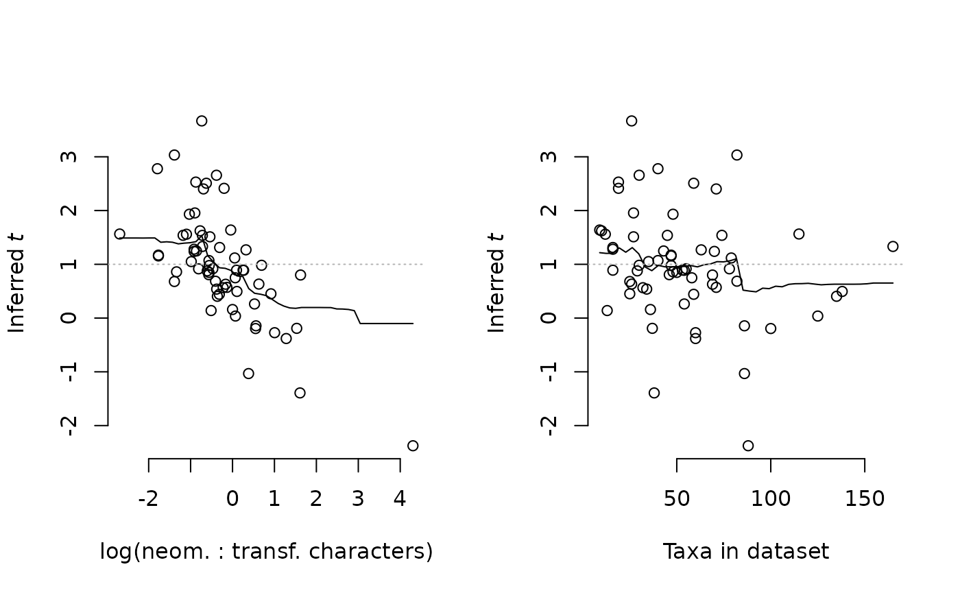
## logNTRatio, nChar, nTaxa
rfT <- randomForest(metaT[, predT, drop = FALSE], t50, ntree = 10000,
                    importance = TRUE)

par(mfrow = c(1, 2))
plot(t50 ~ metaT$logNTRatio, frame.plot = FALSE,
     xlab = Decrypt("logNTRatio"),
     main = "",
     ylab = expression("Inferred" ~ italic("t")))
partialPlot(rfT, metaT, logNTRatio, rug = FALSE, add = TRUE)
abline(h = 1, lty = "dotted", col = "grey70")

plot(t50 ~ metaT$nTaxa, frame.plot = FALSE,
     xlab = Decrypt("nTaxa"),
     main = "",
     ylab = expression("Inferred" ~ italic("t")))
partialPlot(rfT, metaT, nTaxa, rug = FALSE, add = TRUE)
abline(h = 1, lty = "dotted", col = "grey70")
# Compare estimated values of n
bestNModel <- ifelse(marginals["by_n_ki", ] > marginals["by_nt_ki", ],
                     "by_n_ki", "by_nt_ki")

# Estimated value of n using the best available stationary model
# Strictly, this vector stores 1 / n, i.e. rate_loss not rate_gain
stationaryN <- sapply(KiProjects(), function(pID) {
  res <- ExistingResults(pID, bestNModel[pID],
                         checkRemote = FALSE)[["parameters"]][, "rate_loss"]
  if (is.null(res)) {
    message("Need results for ", pID, "_", bestNModel[pID])
    RevBayes(pID, bestNModel[pID])
    MakeSlurm(pID, bestNModel[pID], ml = FALSE)
  }
  res %||% setNames(rep(NA, 6), c("2.5%", "25%", "50%", "75%", "97.5%", "mad"))
})

n50 <- 1 / stationaryN["50%", ]
nModelBF <- ifelse(bestNModel == "by_n_ki",
                   marginals["by_n_ki", ] - marginals["by_ki", ],
                   marginals["by_nt_ki", ] - marginals["by_t_ki", ])

# Which variables predict support for a model with a free n?
nProj <- KiProjects()
nMeta <- data.frame(
  nModelBF,
  nChar = colSums(.meta$nChar[, nProj]),
  nTrans = .meta$nChar["trans", nProj],
  nNeo = .meta$nChar["neo", nProj],
  logNTRatio = log(.meta$nChar["neo", nProj] / .meta$nChar["trans", nProj]),
  charPerTax = colSums(.meta$nChar[, nProj]) / .meta$nTaxa[nProj],
  taxon = .meta$taxon[nProj],
  rank = .meta$rank[nProj],
  nTaxa = .meta$nTaxa[nProj],
  inferredN = 1 / t(stationaryN[, nProj]),
  inferredLogN = -log(t(stationaryN[, nProj]))
)

nPredictors <- c("nChar", "logNTRatio", "charPerTax", "taxon", "rank", "nTaxa",
                 "inferredLogN.50.")
nVsurfBF <- VSURF::VSURF(nMeta[, nPredictors], nModelBF, verbose = FALSE)

nPredBF <- nPredictors[nVsurfBF[["varselect.interp"]]]
message(paste0(nPredBF, collapse = ", "))
## inferredLogN.50., nChar, logNTRatio
nRFBF <- randomForest(nMeta[, nPredBF, drop = FALSE], nModelBF,
                      ntree = 10000, importance = TRUE)
nImp <- importance(nRFBF)
nIncMSE <- nImp[, "%IncMSE"]
nNPred <- length(nPredBF)

par(mfrow = c(ceiling(nNPred / 3), min(3, nNPred)))
for (predictor in nPredBF[order(nIncMSE, decreasing = TRUE)]) {
  plot(nModelBF ~ nMeta[, predictor], frame.plot = FALSE,
       xlab = Decrypt(predictor),
       ylab = lbfLab)
  EpsLine()
  partialPlot(nRFBF, nMeta[, nPredictors], as.character(predictor),
              rug = FALSE, add = TRUE)
}

metaN <- nMeta[!is.na(nMeta[, "inferredN.50."]), ]
ln50 <- metaN[, "inferredLogN.50."]
nvPredictors <- setdiff(nPredictors, c("inferredN.50.", "inferredLogN.50."))
vsurfN <- VSURF::VSURF(metaN[, nvPredictors], ln50, verbose = FALSE)
predN <- nPredictors[vsurfN[["varselect.interp"]]]

cat(paste(predN, collapse = ", "))
## logNTRatio, nChar
sMarginals <- marginals[sub("ns_", "by_", predNS), ]
nsMarginals <- marginals[predNS, ]
bestS <- apply(sMarginals, 2, which.max)
bestNS <- apply(nsMarginals, 2, which.max)

bestML_S  <- marginals[cbind(predS[bestS], colnames(marginals))]
bestML_NS <- marginals[cbind(predNS[bestNS], colnames(marginals))]

stdErr <- attr(marginals, "stdErr")
bestSE_S  <- stdErr[cbind(sub("ns_", "by_", predNS)[bestS], colnames(stdErr))]
bestSE_NS <- stdErr[cbind(predNS[bestNS], colnames(stdErr))]

# Take parameter values from the best non-stationary and stationary models
nsModelBF <- bestML_NS - bestML_S |> `names<-`(colnames(marginals))
nullParam <- c(`2.5%` = NA_real_, `25%` = NA_real_, `50%` = NA_real_,
               `75%` = NA_real_, `97.5%` = NA_real_, mad = NA_real_)

nsValue <- sapply(seq_along(bestS), function(i) {
  ExistingResults(names(bestNS)[i], predNS[bestNS[i]]
  )[["parameters"]][, "root_freqs.1."] %||% nullParam
}) |> `colnames<-`(names(bestS))

# Is the median root frequency different from zero?
# For results that include also ns_t_ki, see 5_Parameters.R
# The values there are used for publication
ns50 <- nsValue["50%", ]
a0 <- nsValue / (1 - nsValue)

# Can we predict which projects will benefit from a non-stationary model?
nsProj <- intersect(colnames(marginals), names(bestS)[!is.na(nsValue[1, ])])
metaA <- data.frame(
  nsModelBF = nsModelBF[nsProj],
  nChar = colSums(.meta$nChar[, nsProj]),
  nTrans = .meta$nChar["trans", nsProj],
  nNeo = .meta$nChar["neo", nsProj],
  logNTRatio = log(.meta$nChar["neo", nsProj] / .meta$nChar["trans", nsProj]),
  charPerTax = colSums(.meta$nChar[, nsProj]) / .meta$nTaxa[nsProj],
  rank = .meta$rank[nsProj],
  taxon = .meta$taxon[nsProj],
  nTaxa = .meta$nTaxa[nsProj],
  # nsValue = t(nsValue[, nsProj]), --> a0Value
  inferredA0.50. = nsValue["50%", nsProj] / (1 - nsValue["50%", nsProj]),
  inferredLogA0.50. = log(nsValue["50%", nsProj] / (1 - nsValue["50%", nsProj]))
)

aPredictors <- c("nChar", "logNTRatio", "charPerTax", "rank",
                 "taxon", "nTaxa", "inferredLogA0.50.")
avPredictors <- setdiff(aPredictors, "inferredLogA0.50.")
a50 <- metaA[, "inferredA0.50."]
la50 <- metaA[, "inferredLogA0.50."]
vsurfA <- VSURF::VSURF(metaA[, avPredictors], la50, verbose = FALSE)
predA <- aPredictors[vsurfA[["varselect.interp"]]]
aVsurfBF <- VSURF::VSURF(metaA[, aPredictors], nsModelBF, verbose = FALSE)
aPredBF <- aPredictors[aVsurfBF[["varselect.interp"]]]
margins <- c(6, 4, 1.4, 0.4)

tvPredictors <- setdiff(tPredictors, "tValue.50.")
predT
## [1] "logNTRatio" "nChar" "nTaxa"
metaTVPred <- metaT[, tvPredictors]
prfTV <- randomForest(metaTVPred, t50, ntree = 10000, importance = TRUE)
OutputPlot("predict_t_val", 7.2, 6, function() {
  par(mfrow = c(2, 3), mar = margins)
  for (predictor in tvPredictors[order(importance(prfTV)[, "%IncMSE"],
                                       decreasing = TRUE)]) {
    PredictWith(metaTVPred, predictor, t50, prfTV, predictor %in% predT,
                expression("Inferred log " ~ italic("t")))
  }
})
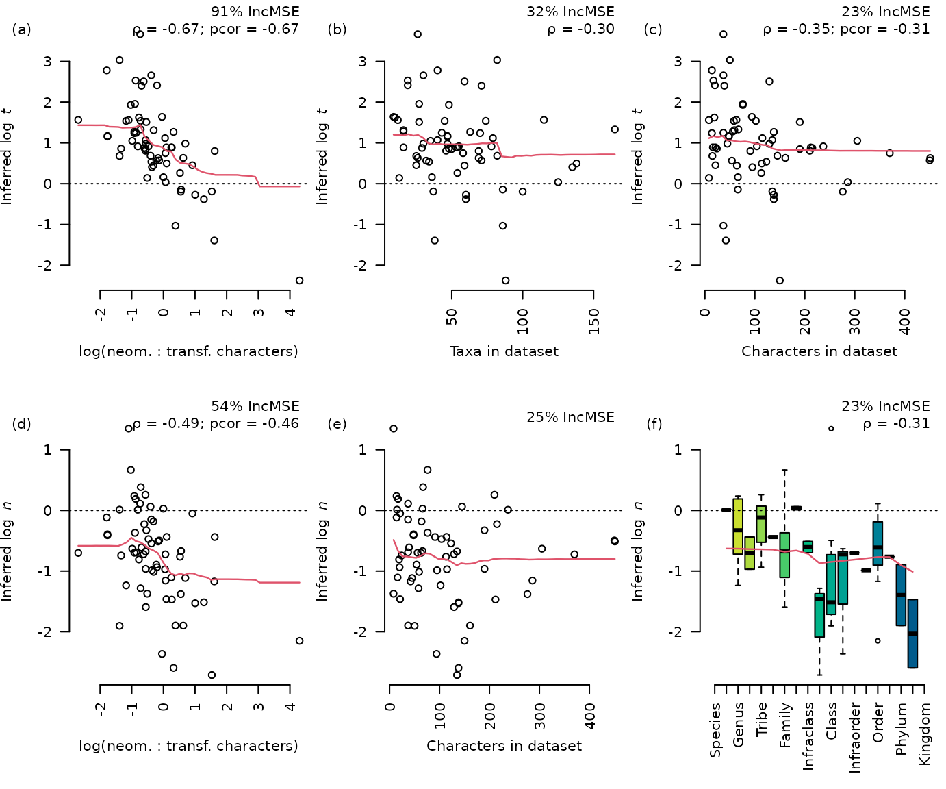
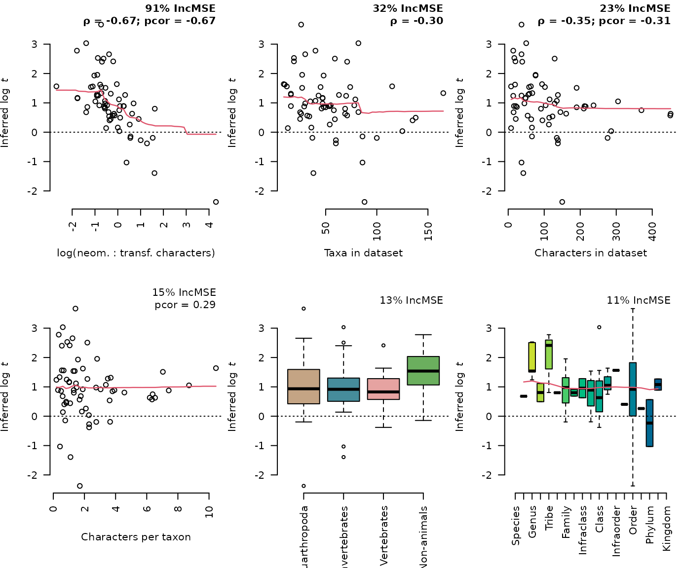
## logNTRatio: Correlated (p = 1e-09): Spearman's rank correlation rho ~ -0.67
## ... Correlated (p = 5.5e-09): pcor ~ -0.67
## nTaxa: Correlated (p = 0.017): Spearman's rank correlation rho ~ -0.3
## ... No significant partial correlation
## nChar: Correlated (p = 0.0051): Spearman's rank correlation rho ~ -0.35
## ... Correlated (p = 0.018): pcor ~ -0.31
## charPerTax: No significant correlation
## ... Correlated (p = 0.025): pcor ~ 0.29
## Warning in xy.coords(x, y): NAs introduced by coercion
## taxon: No significant correlation
## rank: No significant correlation
## ... No significant partial correlation
## [1] "logNTRatio" "nChar"
metaNVPred <- metaN[, nvPredictors]
prfNV <- randomForest(metaNVPred, ln50, ntree = 10000, importance = TRUE)
OutputPlot("predict_n_val", 7.2, 6, function() {
  par(mfrow = c(2, 3), mar = margins)
  for (predictor in nvPredictors[order(importance(prfNV)[, "%IncMSE"],
                                       decreasing = TRUE)]) {
    PredictWith(metaNVPred, predictor, ln50, prfNV, predictor %in% predN,
                expression("Inferred log " ~ italic("n")))
  }
})
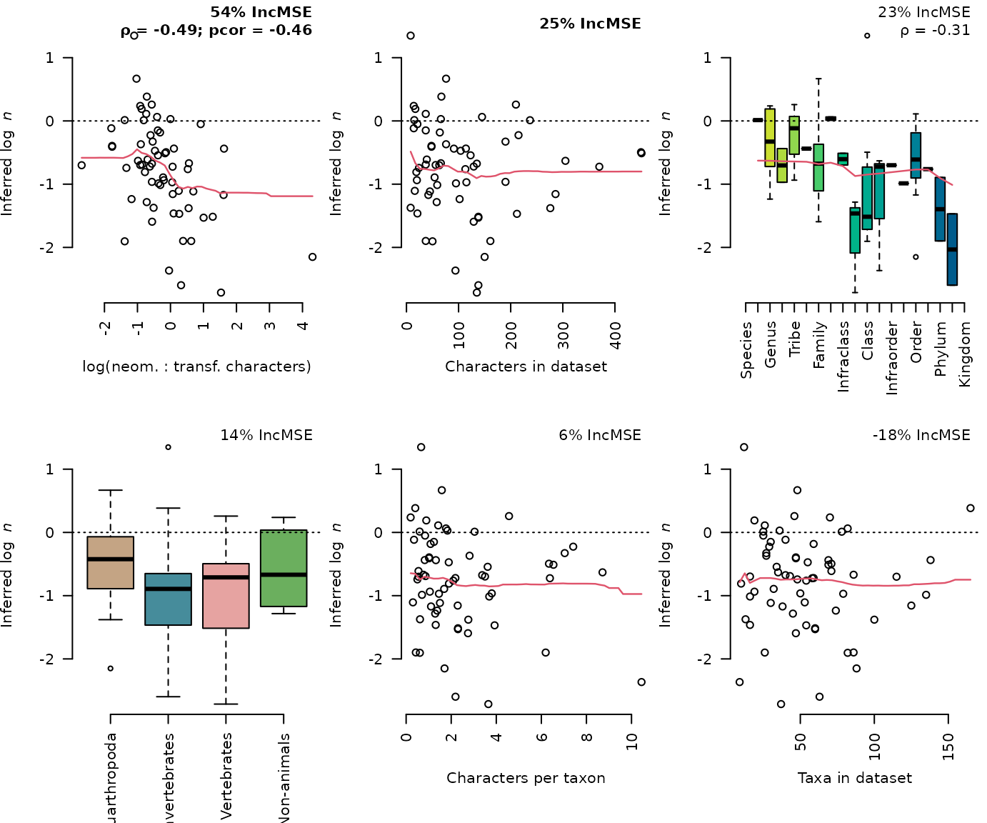
## logNTRatio: Correlated (p = 4.1e-05): Spearman's rank correlation rho ~ -0.49
## ... Correlated (p = 0.00025): pcor ~ -0.46
## nChar: No significant correlation
## ... No significant partial correlation
## rank: Correlated (p = 0.012): Spearman's rank correlation rho ~ -0.31
## ... No significant partial correlation
## Warning in xy.coords(x, y): NAs introduced by coercion
## taxon: No significant correlation
## charPerTax: No significant correlation
## ... No significant partial correlation
## nTaxa: No significant correlation
## ... No significant partial correlation
## [1] "logNTRatio" "nChar"
metaAVPred <- metaA[, avPredictors]
prfAV <- randomForest(metaAVPred, a50, ntree = 10000, importance = TRUE)
OutputPlot("predict_a_val", 7.2, 6, function() {
  par(mfrow = c(2, 3), mar = margins)
  for (predictor in avPredictors[order(importance(prfAV)[, "%IncMSE"],
                                       decreasing = TRUE)]) {
    PredictWith(metaAVPred, predictor, a50, prfAV, predictor %in% predA,
                expression("Inferred log " ~ italic("a")[0]))
  }
})
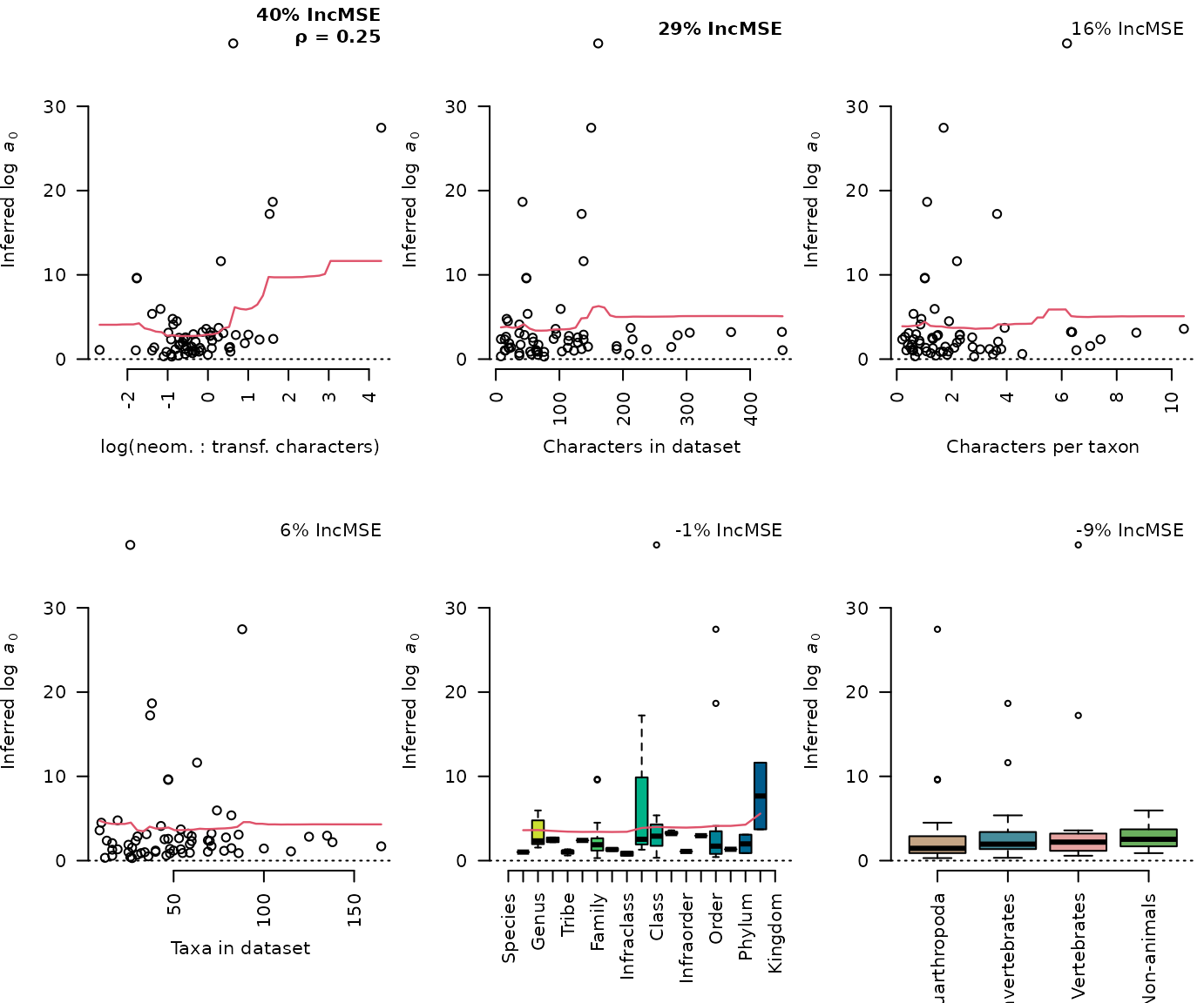
## logNTRatio: Correlated (p = 0.049): Spearman's rank correlation rho ~ 0.25
##       ... No significant partial correlation
## nChar: No significant correlation
## ... No significant partial correlation
## charPerTax: No significant correlation
## ... No significant partial correlation
## nTaxa: No significant correlation
## ... No significant partial correlation
## rank: No significant correlation
## ... No significant partial correlation
## Warning in xy.coords(x, y): NAs introduced by coercion
## taxon: No significant correlation
## [1] "tValue.50." "nChar" "logNTRatio"
metaTPred <- metaT[, tPredictors]
tPredBF
## [1] "tValue.50." "nChar" "logNTRatio"
prfT <- randomForest(metaTPred, tModelBF, ntree = 10000, importance = TRUE)
OutputPlot("predict_t_bf", 7.2, 5, function() {
  par(mfrow = c(2, 4), mar = margins)
  for (predictor in tPredictors[order(importance(prfT)[, "%IncMSE"],
                                      decreasing = TRUE)]) {
    PredictWith(metaTPred, predictor, tModelBF, prfT, predictor %in% tPredBF,
                ylab = lbfLab)
  }
})
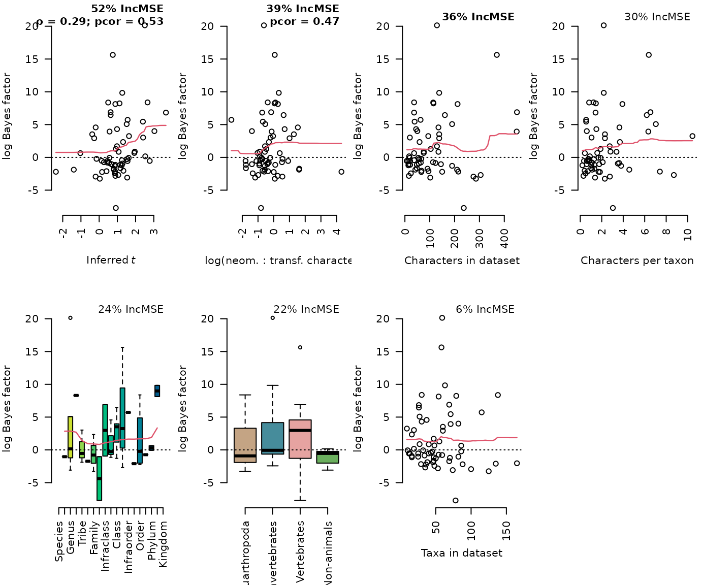
## tValue.50.: Correlated (p = 0.019): Spearman's rank correlation rho ~ 0.29
## ... Correlated (p = 1.3e-05): pcor ~ 0.53
## logNTRatio: No significant correlation
## ... Correlated (p = 0.00015): pcor ~ 0.47
## nChar: No significant correlation
## ... No significant partial correlation
## charPerTax: No significant correlation
## ... No significant partial correlation
## rank: No significant correlation
## ... No significant partial correlation
## Warning in xy.coords(x, y): NAs introduced by coercion
## taxon: No significant correlation
## nTaxa: No significant correlation
## ... No significant partial correlation
metaNPred <- metaN[, nPredictors]
prfN <- randomForest(metaNPred, nModelBF, ntree = 10000, importance = TRUE)
nPredBF
## [1] "inferredLogN.50." "nChar" "logNTRatio"
OutputPlot("predict_n_bf", 7.2, 5, function() {
  par(mfrow = c(2, 4), mar = margins)
  for (predictor in nPredictors[order(importance(prfN)[, "%IncMSE"],
                                      decreasing = TRUE)]) {
    PredictWith(metaNPred, predictor, nModelBF, prfN, predictor %in% nPredBF,
                ylab = lbfLab)
  }
})
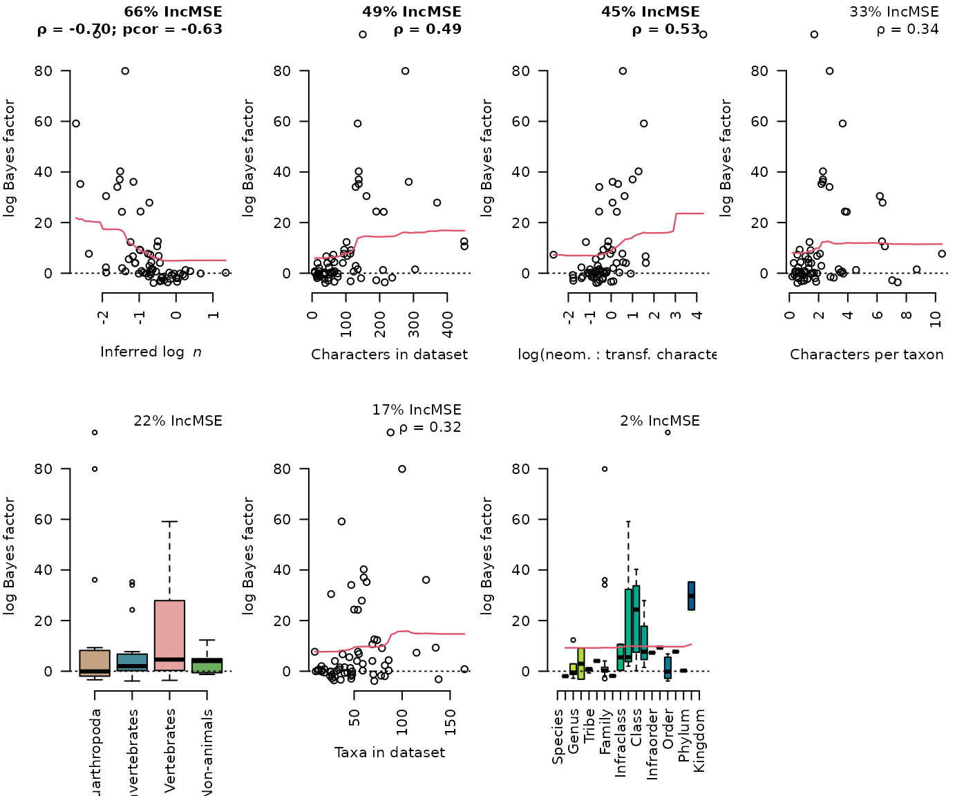
## inferredLogN.50.: Correlated (p = 0): Spearman's rank correlation rho ~ -0.7
## ... Correlated (p = 1.1e-07): pcor ~ -0.63
## nChar: Correlated (p = 4.6e-05): Spearman's rank correlation rho ~ 0.49
## ... No significant partial correlation
## logNTRatio: Correlated (p = 6.5e-06): Spearman's rank correlation rho ~ 0.53
## ... No significant partial correlation
## charPerTax: Correlated (p = 0.006): Spearman's rank correlation rho ~ 0.34
## ... No significant partial correlation
## Warning in xy.coords(x, y): NAs introduced by coercion
## taxon: No significant correlation
## nTaxa: Correlated (p = 0.0098): Spearman's rank correlation rho ~ 0.32
## ... No significant partial correlation
## rank: No significant correlation
## ... No significant partial correlation
metaAPred <- metaA[, aPredictors]
prfA <- randomForest(metaAPred, nsModelBF, ntree = 10000, importance = TRUE)
aPredBF
## [1] "logNTRatio"        "charPerTax"        "nChar"
## [4] "inferredLogA0.50." "taxon"
OutputPlot("predict_a_bf", 7.2, 5, function() {
  par(mfrow = c(2, 4), mar = margins)
  for (predictor in aPredictors[order(importance(prfA)[, "%IncMSE"],
                                      decreasing = TRUE)]) {
    PredictWith(metaAPred, predictor, nsModelBF, prfA, predictor %in% aPredBF,
                ylab = lbfLab)
  }
})
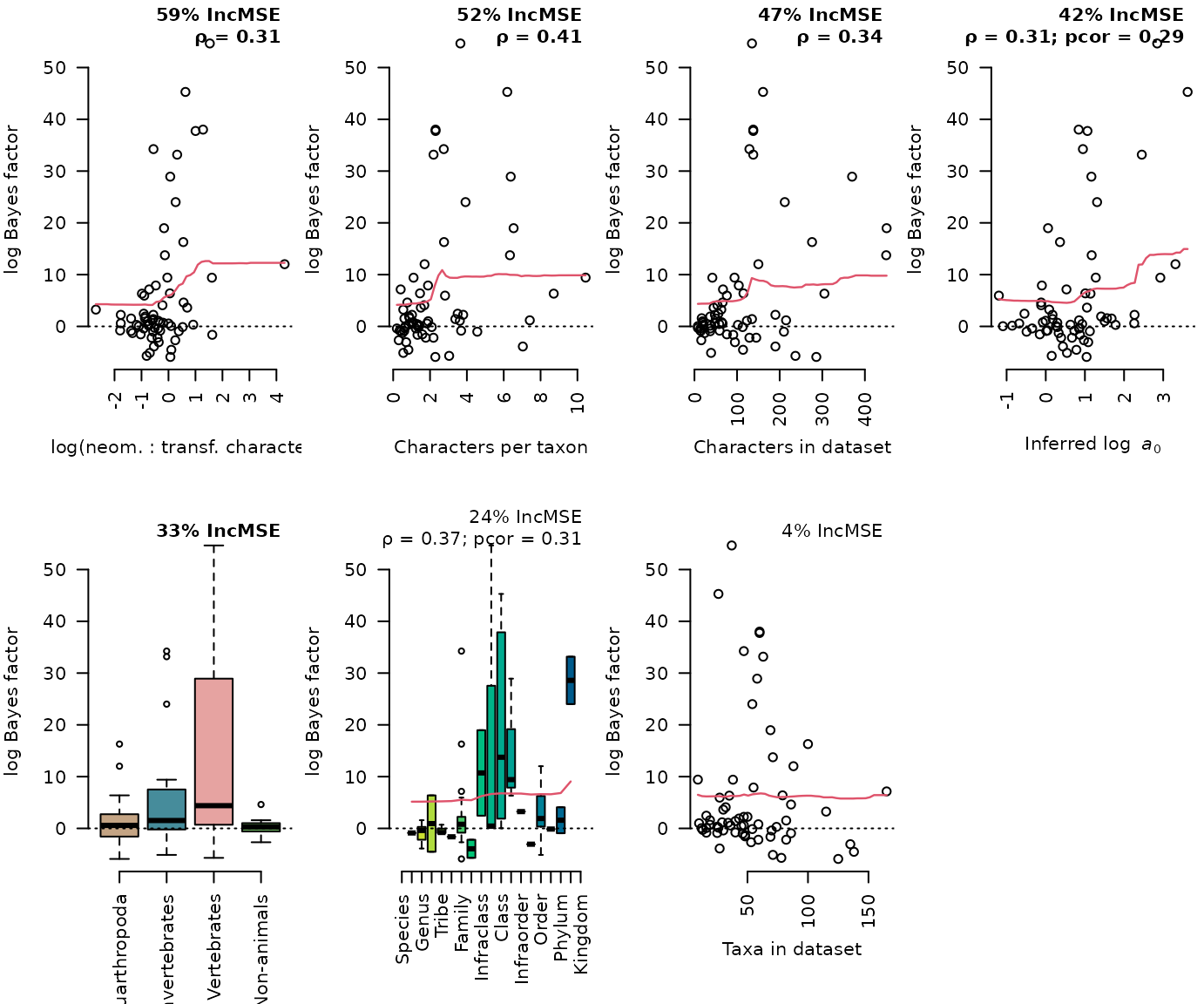
## logNTRatio: Correlated (p = 0.014): Spearman's rank correlation rho ~ 0.31
##       ... No significant partial correlation
## charPerTax: Correlated (p = 0.00086): Spearman's rank correlation rho ~ 0.41
## ... No significant partial correlation
## nChar: Correlated (p = 0.0062): Spearman's rank correlation rho ~ 0.34
## ... No significant partial correlation
## inferredLogA0.50.: Correlated (p = 0.013): Spearman's rank correlation rho ~ 0.31
## ... Correlated (p = 0.024): pcor ~ 0.29
## Warning in xy.coords(x, y): NAs introduced by coercion
## taxon: No significant correlation
## rank: Correlated (p = 0.0029): Spearman's rank correlation rho ~ 0.37
## ... Correlated (p = 0.018): pcor ~ 0.31
## nTaxa: No significant correlation
## ... No significant partial correlation
OutputPlot("predicting_nt", 7.2, 6, function() {
  par(mfrow = c(2, 3), mar = margins)
  panel <- 0
  for (predictor in tvPredictors[order(importance(prfTV)[, "%IncMSE"],
                                       decreasing = TRUE)][1:3]) {
    PredictWith(metaTVPred, predictor, t50, prfTV, FALSE,
                expression("Inferred log " ~ italic("t")))
    Panel(panel <- panel + 1)
  }
  for (predictor in nvPredictors[order(importance(prfNV)[, "%IncMSE"],
                                       decreasing = TRUE)][1:3]) {
    PredictWith(metaNVPred, predictor, ln50, prfNV, FALSE,
                expression("Inferred log " ~ italic("n")))
    Panel(panel <- panel + 1)
  }
})
## logNTRatio: Correlated (p = 1e-09): Spearman's rank correlation rho ~ -0.67
## ... Correlated (p = 5.5e-09): pcor ~ -0.67
## nTaxa: Correlated (p = 0.017): Spearman's rank correlation rho ~ -0.3
## ... No significant partial correlation
## nChar: Correlated (p = 0.0051): Spearman's rank correlation rho ~ -0.35
## ... Correlated (p = 0.018): pcor ~ -0.31
## logNTRatio: Correlated (p = 4.1e-05): Spearman's rank correlation rho ~ -0.49
## ... Correlated (p = 0.00025): pcor ~ -0.46
## nChar: No significant correlation
## ... No significant partial correlation
## rank: Correlated (p = 0.012): Spearman's rank correlation rho ~ -0.31
## ... No significant partial correlation